12.1 Revisiting the disaster framing study
Here we load a couple necessary packages, load the data, and take a glimpse().
library(tidyverse)

disaster <- read_csv("data/disaster/disaster.csv")

glimpse(disaster)
## Observations: 211
## Variables: 5
## $ id <int> 1, 2, 3, 4, 5, 6, 7, 8, 9, 10, 11, 12, 13, 14, 15, 16, 17, 18, 19, 20, 21, 22, 23, 24, 25...
## $ frame <int> 1, 1, 1, 1, 1, 0, 0, 1, 0, 0, 1, 1, 0, 0, 1, 1, 1, 1, 0, 0, 1, 0, 1, 0, 1, 1, 0, 0, 0, 1,...
## $ donate <dbl> 5.6, 4.2, 4.2, 4.6, 3.0, 5.0, 4.8, 6.0, 4.2, 4.4, 5.8, 6.2, 6.0, 4.2, 4.4, 5.8, 5.4, 3.4,...
## $ justify <dbl> 2.95, 2.85, 3.00, 3.30, 5.00, 3.20, 2.90, 1.40, 3.25, 3.55, 1.55, 1.60, 1.65, 2.65, 3.15,...
## $ skeptic <dbl> 1.8, 5.2, 3.2, 1.0, 7.6, 4.2, 4.2, 1.2, 1.8, 8.8, 1.0, 5.4, 2.2, 3.6, 7.8, 1.6, 1.0, 6.4,...Load brms.
library(brms)model1 is the simple moderation model.
model1 <-
  brm(data = disaster, family = gaussian,
      donate ~ 1 + frame + skeptic + frame:skeptic,
      chains = 4, cores = 4)
Our model1 summary matches nicely with the text.
print(model1, digits = 3)## Family: gaussian
## Links: mu = identity; sigma = identity
## Formula: donate ~ 1 + frame + skeptic + frame:skeptic
## Data: disaster (Number of observations: 211)
## Samples: 4 chains, each with iter = 2000; warmup = 1000; thin = 1;
## total post-warmup samples = 4000
##
## Population-Level Effects:
## Estimate Est.Error l-95% CI u-95% CI Eff.Sample Rhat
## Intercept 5.029 0.228 4.584 5.479 2070 1.002
## frame 0.681 0.335 0.014 1.333 1969 1.001
## skeptic -0.139 0.058 -0.255 -0.025 1949 1.003
## frame:skeptic -0.171 0.085 -0.341 0.003 1816 1.002
##
## Family Specific Parameters:
## Estimate Est.Error l-95% CI u-95% CI Eff.Sample Rhat
## sigma 1.240 0.062 1.124 1.366 2855 1.001
##
## Samples were drawn using sampling(NUTS). For each parameter, Eff.Sample
## is a crude measure of effective sample size, and Rhat is the potential
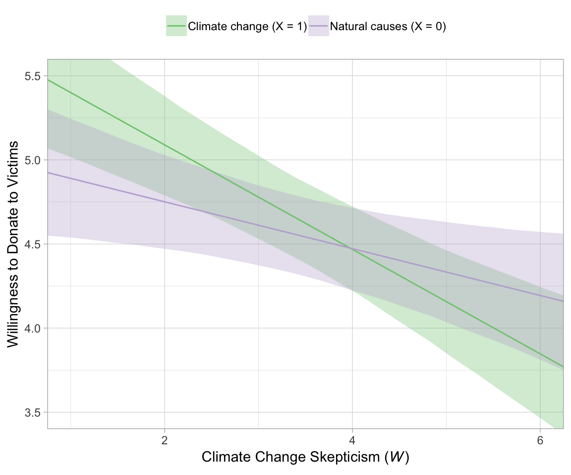
## scale reduction factor on split chains (at convergence, Rhat = 1).For the figures in this chapter, we’ll take theme cues from Matthew Kay’s tidybayes package. Otherwise, our Figure 12.2 is business as usual at this point.
theme_set(theme_light())

nd <-
  tibble(frame = rep(0:1, each = 30),
         skeptic = rep(seq(from = 0, to = 7, length.out = 30),
                       times = 2))

fitted(model1, newdata = nd) %>%
  as_tibble() %>%
  bind_cols(nd) %>%
  mutate(frame = ifelse(frame == 0, str_c("Natural causes (X = ", frame, ")"),
                        str_c("Climate change (X = ", frame, ")"))) %>%

  ggplot(aes(x = skeptic, y = Estimate)) +
  geom_ribbon(aes(ymin = Q2.5, ymax = Q97.5, fill = frame),
              alpha = 1/3) +
  geom_line(aes(color = frame)) +
  scale_fill_brewer(type = "qual") +
  scale_color_brewer(type = "qual") +
  coord_cartesian(xlim = 1:6,
                  ylim = c(3.5, 5.5)) +
  labs(x = expression(paste("Climate Change Skepticism (", italic(W), ")")),
       y = "Willingness to Donate to Victims") +
  theme(legend.position = "top",
        legend.direction = "horizontal",
        legend.title = element_blank())
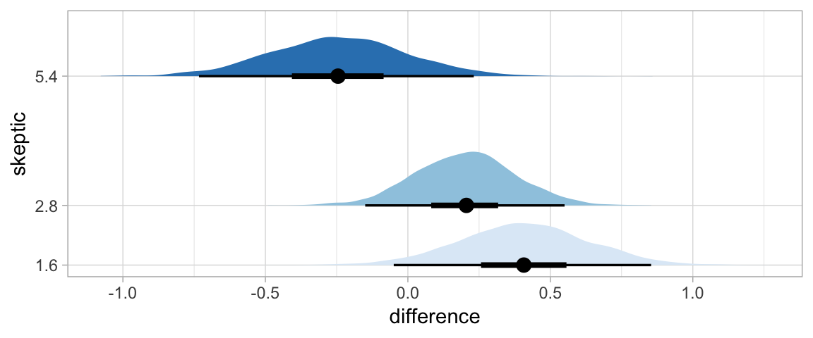
In Hayes’s Figure 12.2, he emphasized the differences at the three levels of skeptic. If you want the full difference score distributions in a pick-a-point-approach sort of way, you might plot the densities with tidybayes::geom_halfeyeh(), which places coefficient plots at the base of the densities. In this case, we show the posterior medians with the dots, the 50% intervals with the thick horizontal lines, and the 95% intervals with the thinner horizontal lines.
library(tidybayes)
nd <-
  tibble(frame = rep(0:1, times = 3),
         skeptic = rep(quantile(disaster$skeptic, probs = c(.16, .5, .86)),
                                times = 2))

fitted(model1, summary = F,
       newdata = nd) %>%
  as_tibble() %>%
  gather() %>%
  mutate(frame = rep(rep(0:1, times = 3),
                     each = 4000),
         skeptic = rep(rep(quantile(disaster$skeptic, probs = c(.16, .5, .86)),
                                times = 2),
                       each = 4000),
         iter = rep(1:4000, times = 6)) %>%
  select(-key) %>%
  spread(key = frame, value = value) %>%
  mutate(difference = `1` - `0`) %>%

  ggplot(aes(x = difference, y = skeptic, fill = skeptic %>% as.character())) +
  geom_halfeyeh(point_interval = median_qi, .prob = c(0.95, 0.5)) +
  scale_fill_brewer() +
  scale_y_continuous(breaks = quantile(disaster$skeptic, probs = c(.16, .5, .86)),
                     labels = quantile(disaster$skeptic, probs = c(.16, .5, .86)) %>% round(2)) +
  theme(legend.position = "none",
        panel.grid.minor.y = element_blank())
Here’s our simple mediation model, model2, using the multivariate syntax right in the brm() function.
model2 <-
  brm(data = disaster, family = gaussian,
      bf(justify ~ 1 + frame) +
        bf(donate ~ 1 + frame + justify) +
        set_rescor(FALSE),
chains = 4, cores = 4)print(model2, digits = 3)## Family: MV(gaussian, gaussian)
## Links: mu = identity; sigma = identity
## mu = identity; sigma = identity
## Formula: justify ~ 1 + frame
## donate ~ 1 + frame + justify
## Data: disaster (Number of observations: 211)
## Samples: 4 chains, each with iter = 2000; warmup = 1000; thin = 1;
## total post-warmup samples = 4000
##
## Population-Level Effects:
## Estimate Est.Error l-95% CI u-95% CI Eff.Sample Rhat
## justify_Intercept 2.801 0.091 2.619 2.981 4000 1.000
## donate_Intercept 7.235 0.233 6.776 7.688 4000 0.999
## justify_frame 0.134 0.127 -0.116 0.379 4000 1.000
## donate_frame 0.211 0.135 -0.060 0.480 4000 1.000
## donate_justify -0.954 0.076 -1.102 -0.805 4000 0.999
##
## Family Specific Parameters:
## Estimate Est.Error l-95% CI u-95% CI Eff.Sample Rhat
## sigma_justify 0.935 0.045 0.850 1.026 4000 1.000
## sigma_donate 0.987 0.049 0.898 1.090 4000 0.999
##
## Samples were drawn using sampling(NUTS). For each parameter, Eff.Sample
## is a crude measure of effective sample size, and Rhat is the potential
## scale reduction factor on split chains (at convergence, Rhat = 1).Consider the Bayesian \(R^2\) summaries.
bayes_R2(model2) %>% round(digits = 3)## Estimate Est.Error Q2.5 Q97.5
## R2_justify 0.010 0.011 0.000 0.040
## R2_donate 0.449 0.039 0.367 0.519If you want the indirect effect with its intervals, you use posterior_samples() and data wrangle, as usual.
posterior_samples(model2) %>%
  mutate(ab = b_justify_frame*b_donate_justify) %>%
  summarize(mean = mean(ab),
            ll = quantile(ab, probs = .025),
            ul = quantile(ab, probs = .975)) %>%
  mutate_if(is.double, round, digits = 3)
## mean ll ul
## 1 -0.128 -0.364 0.11We might also streamline our code a touch using tidybayes::mean_qi() in place of tidyverse::summarize().
posterior_samples(model2) %>%
  mutate(ab = b_justify_frame*b_donate_justify) %>%
  mean_qi(ab, .prob = .95) %>%
  mutate_if(is.double, round, digits = 3)
## # A tibble: 1 x 4
## ab conf.low conf.high .prob
## <dbl> <dbl> <dbl> <dbl>
## 1 -0.128 -0.364 0.11 0.95Note that the last column explicates what interval level we used.