11.6 Statistical inference
11.6.1 Inference about the direct effect.
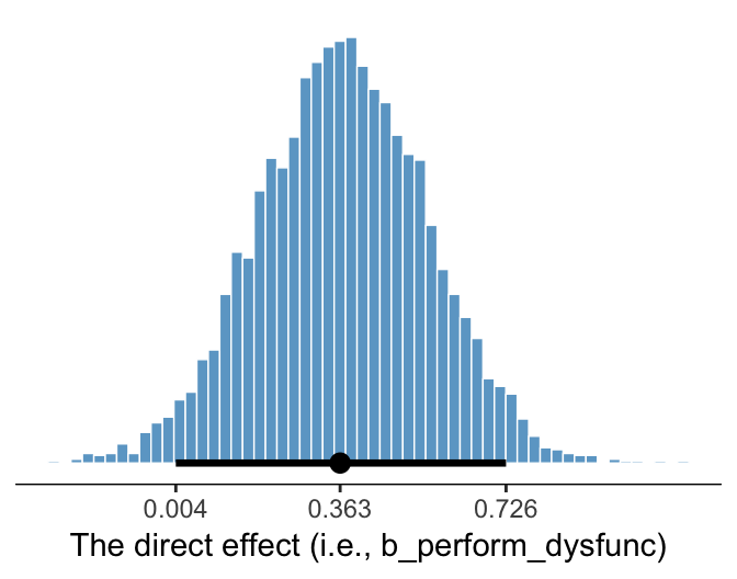
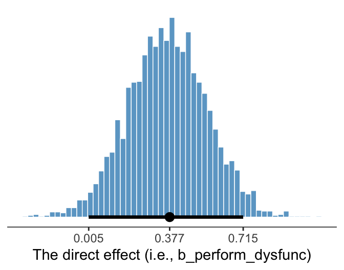
We’ve already seen the 95% percentile-based crecible intervals for the direct effect, b_perform_dysfunc, which we can get with print(), posterior_summary(), or even fixef(). Here we’ll go beyond summaries and plot using geom_histogram().
library(tidybayes)

post %>%
  ggplot(aes(x = b_perform_dysfunc)) +
  geom_histogram(binwidth = .025, boundary = 0,
                 color = "white", fill = "skyblue3", size = 1/4) +
  stat_pointintervalh(aes(y = 0),
                      point_interval = mode_hdi, .prob = .95) +
  scale_x_continuous(breaks = mode_hdi(post$b_perform_dysfunc, .prob = .95)[1, 1:3],
                     labels = mode_hdi(post$b_perform_dysfunc, .prob = .95)[1, 1:3] %>% round(3)) +
  scale_y_continuous(NULL, breaks = NULL) +
  xlab("The direct effect (i.e., b_perform_dysfunc)") +
  theme_bw() +
  theme(panel.grid = element_blank(),
        panel.border = element_blank(),
        axis.line.x = element_line(size = 1/4))
Since we’re plotting in a style similar to Kruschke, we switched from emphasizing the posterior mean or median to marking off the posterior mode, which is Kruschkes’ preferred metric of central tendency. We also ditched our typical percentile-based 95% intervals for highest posterior density intervals. The stat_pointintervalh() function from the Matthew Kay’s tidybayes package made it easy to compute those values with the point_interval = mode_hdi argument. Note how we also used tidybayes::mode_hdi() to compute those values and plug them into scale_x_continuous().
11.6.2 Inference about the indirect effect.
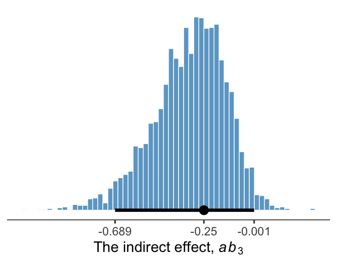
Much like above, we can make a plot of the conditional indirect effect \(ab_{3}\).
post <-
  post %>%
  mutate(ab_3 = b_negtone_dysfunc*`b_perform_negtone:negexp`)

post %>%
  ggplot(aes(x = ab_3)) +
  geom_histogram(binwidth = .025, boundary = 0,
                 color = "white", fill = "skyblue3", size = 1/4) +
  stat_pointintervalh(aes(y = 0),
                      point_interval = mode_hdi, .prob = .95) +
  scale_x_continuous(breaks = mode_hdi(post$ab_3, .prob = .95)[1, 1:3],
                     labels = mode_hdi(post$ab_3, .prob = .95)[1, 1:3] %>% round(3)) +
  scale_y_continuous(NULL, breaks = NULL) +
  xlab(expression(paste("The indirect effect, ", italic(ab)[3]))) +
  theme_bw() +
  theme(panel.grid = element_blank(),
        panel.border = element_blank(),
        axis.line.x = element_line(size = 1/4))
11.6.3 Probing moderation of mediation.
11.6.3.1 Normal theory approach.
As we’re square within the Bayesian modeling paradigm, we have no need to appeal to normal theory for the posterior \(SD\)s or 95% intervals.
11.6.3.2 Bootstrap confidence intervals Two types of Bayesian credible intervals.
We produced the summary values corresponding to those in Table 11.3 some time ago. Here they are, again.
post %>%
  select(starts_with("Conditional indirect")) %>%
  gather() %>%
  mutate(key = factor(key, levels = c("Conditional indirect effect when W is -0.531",
                                      "Conditional indirect effect when W is -0.006",
                                      "Conditional indirect effect when W is 0.600"))) %>%
  group_by(key) %>%
  summarize(mean = mean(value),
            sd = sd(value),
            ll = quantile(value, probs = .025),
            ul = quantile(value, probs = .975)) %>%
  mutate_if(is.double, round, digits = 3)
## # A tibble: 3 x 5
## key mean sd ll ul
## <fct> <dbl> <dbl> <dbl> <dbl>
## 1 Conditional indirect effect when W is -0.531 -0.104 0.141 -0.407 0.165
## 2 Conditional indirect effect when W is -0.006 -0.254 0.114 -0.51 -0.066
## 3 Conditional indirect effect when W is 0.600 -0.464 0.167 -0.824 -0.177Those were our usual percentile-based intervals. If we wanted to summarize those same effects with posterior modes and 95% highest posterior density intervals, instead, we’d replace our summarize() code with a mode_hdi() statement.
post %>%
  select(starts_with("Conditional indirect")) %>%
  gather() %>%
  mutate(key = factor(key, levels = c("Conditional indirect effect when W is -0.531",
                                      "Conditional indirect effect when W is -0.006",
                                      "Conditional indirect effect when W is 0.600"))) %>%
  group_by(key) %>%
  mode_hdi(value, .prob = .95) %>%
  mutate_if(is.double, round, digits = 3)
## # A tibble: 3 x 5
## # Groups: key [3]
## key value conf.low conf.high .prob
## <fct> <dbl> <dbl> <dbl> <dbl>
## 1 Conditional indirect effect when W is -0.531 -0.063 -0.409 0.162 0.95
## 2 Conditional indirect effect when W is -0.006 -0.203 -0.493 -0.052 0.95
## 3 Conditional indirect effect when W is 0.600 -0.431 -0.802 -0.164 0.95And we might plot these with something like:
post %>%
  select(starts_with("Conditional indirect")) %>%
  gather() %>%
  mutate(key = str_remove(key, "Conditional indirect effect when W is ") %>% as.double()) %>%

  ggplot(aes(x = key, y = value, group = key)) +
  stat_pointinterval(point_interval = mode_hdi, .prob = c(.95, .5),
                     color = "skyblue3") +
  scale_x_continuous(breaks = c(-.531, -.006, .6)) +
  coord_cartesian(xlim = c(-.5, .6),
                  ylim = c(-1.25, .75)) +
  labs(x = expression(italic(W)),
       y = "The conditional indirect effect") +
  theme_bw() +
  theme(panel.grid = element_blank())
This time we used the prob = c(.95, .5) argument within stat_pointinterval() to return both 95% and 50% highest posterior density intervals—which are the outer and inner lines, respectively.
This, of course, leads us right into:
11.6.3.3 A Johnson-Neyman approach.
On page 429, Hayes discussed how Preacher et al. (2007)’s attempt to apply the JN technique in this context presumed
the sampling distribution of the conditional indirect effect is normal. Given that the sampling distribution of the conditional indirect effect is not normal, the approach they describe yields, at best, an approximate solution. To [Hayes’s] knowledge, no one has ever proposed a bootstrapping-based analogue of the Johnson-Neyman method for probing the moderation of an indirect effect.
However, our Bayesian HMC approach makes no such assumption. All we need to do is manipulate the posterior as usual. Here it is, this time using all 4000 iterations:
post %>%
  transmute(`-0.8` = b_perform_negtone + `b_perform_negtone:negexp`*-0.8,
            `0.8` = b_perform_negtone + `b_perform_negtone:negexp`*0.8) %>%
  gather() %>%
  mutate(key = key %>% as.double,
         iter = rep(1:4000, times = 2)) %>%

  ggplot(aes(x = key, y = value, group = iter)) +
  geom_line(color = "skyblue3",
            size = 1/6, alpha = 1/15) +
  coord_cartesian(xlim = c(-.5, .6),
                  ylim = c(-1.25, .75)) +
  labs(x = expression(italic(W)),
       y = "The conditional indirect effect") +
  theme_bw() +
  theme(panel.grid = element_blank())