7.2 An example: Climate change disasters and humanitarianism
Here we load a couple necessary packages, load the data, and take a glimpse().
disaster <- read_csv("data/disaster/disaster.csv")

glimpse(disaster)
## Observations: 211
## Variables: 5
## $ id <int> 1, 2, 3, 4, 5, 6, 7, 8, 9, 10, 11, 12, 13, 14, 15, 16, 17, 18, 19, 20, 21, 22, 23, 24, 25...
## $ frame <int> 1, 1, 1, 1, 1, 0, 0, 1, 0, 0, 1, 1, 0, 0, 1, 1, 1, 1, 0, 0, 1, 0, 1, 0, 1, 1, 0, 0, 0, 1,...
## $ donate <dbl> 5.6, 4.2, 4.2, 4.6, 3.0, 5.0, 4.8, 6.0, 4.2, 4.4, 5.8, 6.2, 6.0, 4.2, 4.4, 5.8, 5.4, 3.4,...
## $ justify <dbl> 2.95, 2.85, 3.00, 3.30, 5.00, 3.20, 2.90, 1.40, 3.25, 3.55, 1.55, 1.60, 1.65, 2.65, 3.15,...
## $ skeptic <dbl> 1.8, 5.2, 3.2, 1.0, 7.6, 4.2, 4.2, 1.2, 1.8, 8.8, 1.0, 5.4, 2.2, 3.6, 7.8, 1.6, 1.0, 6.4,...Here is how to get the ungrouped mean and \(SD\) values for justify and skeptic, as presented in Table 7.3.
disaster %>%
  select(justify, skeptic) %>%
  gather() %>%
  group_by(key) %>%
  summarise(mean = mean(value),
            sd = sd(value)) %>%
  mutate_if(is.double, round, digits = 3)
## # A tibble: 2 x 3
## key mean sd
## <chr> <dbl> <dbl>
## 1 justify 2.87 0.93
## 2 skeptic 3.38 2.03And here we get the same summary values, this time grouped by frame.
disaster %>%
  select(frame, justify, skeptic) %>%
  gather(key, value, -frame) %>%
  group_by(frame, key) %>%
  summarise(mean = mean(value),
            sd = sd(value)) %>%
  mutate_if(is.double, round, digits = 3)
## # A tibble: 4 x 4
## # Groups: frame [2]
## frame key mean sd
## <int> <chr> <dbl> <dbl>
## 1 0 justify 2.80 0.849
## 2 0 skeptic 3.34 2.04
## 3 1 justify 2.94 1.01
## 4 1 skeptic 3.42 2.03Let’s open brms.
library(brms)Anticipating Table 7.4 on page 234, we’ll name this first model model1.
model1 <-
  brm(data = disaster, family = gaussian,
      justify ~ 1 + frame,
chains = 4, cores = 4)print(model1)## Family: gaussian
## Links: mu = identity; sigma = identity
## Formula: justify ~ 1 + frame
## Data: disaster (Number of observations: 211)
## Samples: 4 chains, each with iter = 2000; warmup = 1000; thin = 1;
## total post-warmup samples = 4000
##
## Population-Level Effects:
## Estimate Est.Error l-95% CI u-95% CI Eff.Sample Rhat
## Intercept 2.80 0.09 2.63 2.97 3083 1.00
## frame 0.13 0.13 -0.11 0.39 3342 1.00
##
## Family Specific Parameters:
## Estimate Est.Error l-95% CI u-95% CI Eff.Sample Rhat
## sigma 0.94 0.05 0.85 1.03 4000 1.00
##
## Samples were drawn using sampling(NUTS). For each parameter, Eff.Sample
## is a crude measure of effective sample size, and Rhat is the potential
## scale reduction factor on split chains (at convergence, Rhat = 1).The ‘Estimate’ (i.e., posterior mean) of the model intercept is the expected justify value for when frame is 0. The ‘Estimate’ for frame is the expected difference when frame is a 1. If all you care about is the posterior mean, you could do
fixef(model1)["Intercept", 1] + fixef(model1)["frame", 1]## [1] 2.935378which matches up nicely with the equation on page 233. But this wouldn’t be very Bayesian of us. It’d be more satisfying if we had an expression of the uncertainty in the value. For that, we’ll follow our usual practice of extracting the posterior samples, making nicely-named vectors, and summarizing a bit.
post <-
  posterior_samples(model1) %>%
  mutate(when_x_is_0 = b_Intercept,
         when_x_is_1 = b_Intercept + b_frame)

post %>%
  select(when_x_is_0, when_x_is_1) %>%
  gather() %>%
  group_by(key) %>%
  summarize(mean = mean(value),
            sd = sd(value)) %>%
  mutate_if(is.double, round, digits = 3)
## # A tibble: 2 x 3
## key mean sd
## <chr> <dbl> <dbl>
## 1 when_x_is_0 2.80 0.089
## 2 when_x_is_1 2.94 0.092Hayes referenced a \(t\)-test and accompanying \(p\)-value in the lower part of page 233. We, of course, aren’t going to do that. But we do have the 95% intervals in our print() output, above, which we can also look at like so.
posterior_interval(model1)["b_frame", ]## 2.5% 97.5%
## -0.1143789 0.3934074And we can always plot.
post %>%
  ggplot(aes(x = b_frame)) +
  geom_density(size = 0, fill = dutchmasters$little_street[1]) +
  geom_vline(xintercept = 0, color = dutchmasters$little_street[11]) +
  scale_x_continuous(breaks = c(-.3, 0, .6)) +
  scale_y_continuous(NULL, breaks = NULL) +
  theme_07 +
  theme(legend.position = "none")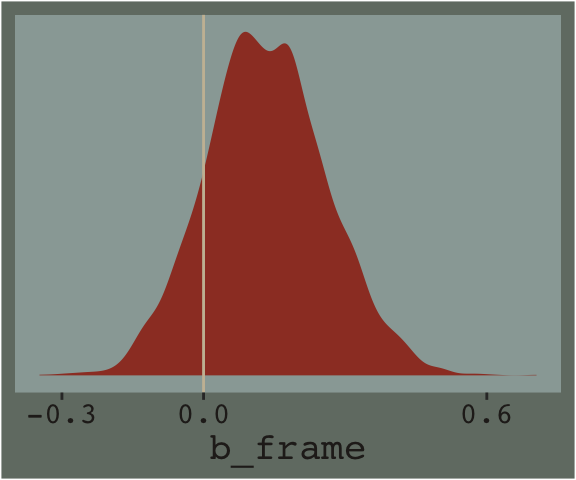
We’ll use the update() function to hastily fit model2 and model3.
model2 <-
  update(model1, newdata = disaster,
         formula = justify ~ 1 + frame + skeptic,
         chains = 4, cores = 4)

model3 <-
  update(model1, newdata = disaster,
         formula = justify ~ 1 + frame + skeptic + frame:skeptic,
         chains = 4, cores = 4)
Note our use of the frame:skeptic syntax in model3. With that syntax we didn’t need to make an interaction variable in the data by hand. The brms package just handled it for us. An alternative syntax would have been frame*skeptic. But if you really wanted to make the interaction variable by hand, you’d do this.
disaster <-
  disaster %>%
  mutate(interaction_variable = frame*skeptic)
Once you have interaction_variable in the data, you’d specify a model formula within the brm() function like formula = justify ~ 1 + frame + skeptic + interaction_variable. I’m not going to do that, here, but you can play around yourself if so inclined.
Here are the quick and dirty coefficient summaries for our two new models.
posterior_summary(model2)## Estimate Est.Error Q2.5 Q97.5
## b_Intercept 2.1307082 0.12777249 1.8829093 2.3891387
## b_frame 0.1169393 0.11481339 -0.1048338 0.3386479
## b_skeptic 0.2011168 0.02921602 0.1444075 0.2557176
## sigma 0.8422032 0.04201156 0.7664790 0.9304656
## lp__ -268.3729553 1.41272791 -271.8371388 -266.5718957posterior_summary(model3)## Estimate Est.Error Q2.5 Q97.5
## b_Intercept 2.4528494 0.14887569 2.1677181 2.7432500
## b_frame -0.5687102 0.21703257 -0.9937620 -0.1406217
## b_skeptic 0.1042967 0.03788573 0.0320306 0.1788565
## b_frame:skeptic 0.2027146 0.05483136 0.0927857 0.3061208
## sigma 0.8176487 0.04040054 0.7433312 0.8996959
## lp__ -262.2631690 1.53602416 -266.1279187 -260.2129900Just focusing on our primary model, model3, here’s another way to look at the coefficients.
stanplot(model3) +
  theme_07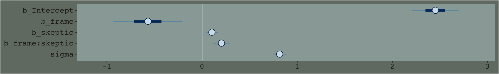
By default, brms::stanplot() makes coefficient plots which depict the parameters of a model by their posterior means (i.e., dots), 50% intervals (i.e., thick horizontal lines), and 95% intervals (i.e., thin horizontal lines). As stanplot() returns a ggplot2 object, one can customize the theme and so forth.
We’ll extract the \(R^2\) iterations in the usual way once for each model, and then combine them for a plot.
# for each of the three models, we create a separare R2 tibble
R2_model1 <-
  bayes_R2(model1,
           summary = F) %>%
  as_tibble()

R2_model2 <-
  bayes_R2(model2,
           summary = F) %>%
  as_tibble()

R2_model3 <-
  bayes_R2(model3,
           summary = F) %>%
  as_tibble()

# here we combine them into one tibble, indexed by `model`
R2s <-
  R2_model1 %>%
  bind_rows(R2_model2) %>%
  bind_rows(R2_model3) %>%
  mutate(model = rep(c("model1", "model2", "model3"), each = 4000))

# now we plot
R2s %>%
  ggplot(aes(x = R2)) +
  geom_density(aes(fill = model), size = 0, alpha = 2/3) +
  scale_fill_manual(NULL,
                    values = dutchmasters$little_street[c(3, 4, 8)] %>% as.character()) +
  scale_y_continuous(NULL, breaks = NULL) +
  xlab(expression(paste(italic(R)^2, " distribution"))) +
  coord_cartesian(xlim = 0:1) +
  theme_07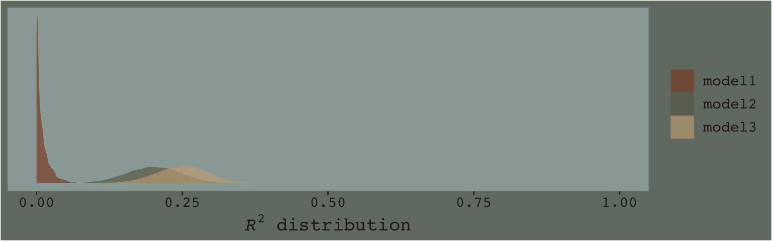
Here’s the \(\Delta R^2\) distribution for model3 minus model2.
R2_model2 %>%
  rename(model2 = R2) %>%
  bind_cols(R2_model3) %>%
  rename(model3 = R2) %>%
  mutate(dif = model3 - model2) %>%

  ggplot(aes(x = dif)) +
  geom_density(color = "transparent",
               fill = dutchmasters$little_street[9]) +
  scale_y_continuous(NULL, breaks = NULL) +
  labs(title = expression(paste("The ", Delta, italic(R)^2)),
       subtitle = "Like in the text, the posterior\nmean is about 0.05.",
       x = NULL) +
  theme_07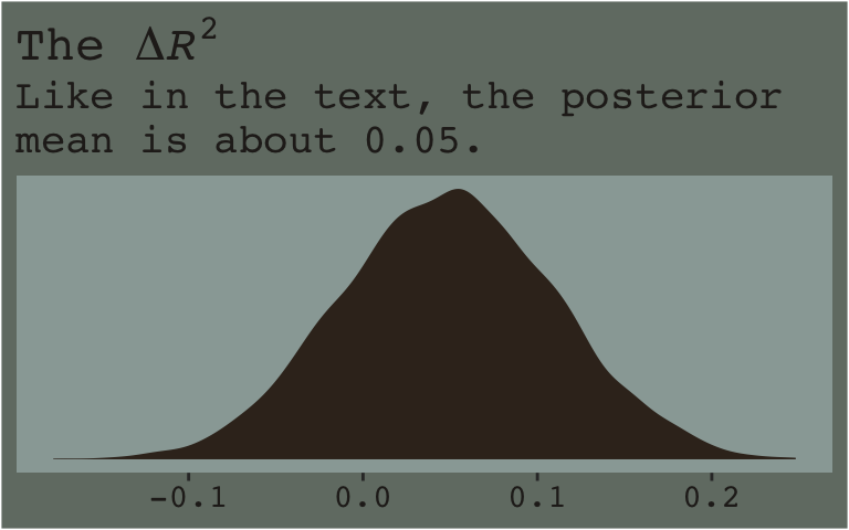
In addition to the \(R^2\), one can use information criteria to compare the models. Here we’ll use the LOO to compare all three.
loo(model1, model2, model3)## LOOIC SE
## model1 572.28 24.03
## model2 529.46 22.37
## model3 517.87 21.69
## model1 - model2 42.82 16.14
## model1 - model3 54.41 18.93
## model2 - model3 11.59 8.29The point estimate for both multivariable models were clearly lower than that for model1. The point estimate for the moderation model, model3, was within the double-digit range lower than that for model2, which typically suggests better fit. But notice how wide the standard error was. There’s a lot of uncertainty, there. Hopefully this isn’t surprising. Our \(R^2\) difference was small and uncertain, too. We can also compare them with AIC-type model weighting, which you can learn more about starting at this point in this lecture or this related vignette for the loo package. Here we’ll keep things simple and weight with the LOO.
model_weights(model1, model2, model3,
              weights = "loo")
## model1 model2 model3
## 1.526031e-12 3.029832e-03 9.969702e-01The model_weights() results put almost all the relative weight on model3. This doesn’t mean model3 is the “true model” or anything like that. It just suggests that it’s the better of the three with respect to the data.
Here are the results of the equations in the second half of page 237.
post <- posterior_samples(model3)

post %>%
  transmute(if_2   = b_frame + `b_frame:skeptic`*2,
            if_3.5 = b_frame + `b_frame:skeptic`*3.5,
            if_5   = b_frame + `b_frame:skeptic`*5) %>%
  gather() %>%
  group_by(key) %>%
  summarise(mean = mean(value),
            sd = sd(value)) %>%
  mutate_if(is.double, round, digits = 3)
## # A tibble: 3 x 3
## key mean sd
## <chr> <dbl> <dbl>
## 1 if_2 -0.163 0.135
## 2 if_3.5 0.141 0.112
## 3 if_5 0.445 0.1427.2.1 Estimation using PROCESS brms.
Similar to what Hayes advertised with PROCESS, with our formula = justify ~ 1 + frame + skeptic + frame:skeptic code in model3, we didn’t need to hard code an interaction variable into the data. brms handled that for us.
7.2.2 Interpreting the regression coefficients.
7.2.3 Variable scaling and the interpretation of \(b_{1}\) and \(b_{3}\).
Making the mean-centered version of our \(W\) variable, skeptic, is a simple mutate() operation. We’ll just call it skeptic_c.
disaster <-
  disaster %>%
  mutate(skeptic_c = skeptic - mean(skeptic))
And here’s how we might fit the model.
model4 <-
  update(model3, newdata = disaster,
         formula = justify ~ 1 + frame + skeptic_c + frame:skeptic_c,
         chains = 4, cores = 4)
Here are the summaries of our fixed effects.
fixef(model4)## Estimate Est.Error Q2.5 Q97.5
## Intercept 2.8053071 0.07760306 2.65492192 2.9598509
## frame 0.1183069 0.11189621 -0.10400167 0.3375879
## skeptic_c 0.1054818 0.03774031 0.03023059 0.1791417
## frame:skeptic_c 0.2013565 0.05505230 0.09431049 0.3095814Here are the \(R^2\) distributions for model3 and model4. They’re the same within simulaiton variance.
bayes_R2(model3) %>% round(digits = 3)## Estimate Est.Error Q2.5 Q97.5
## R2 0.249 0.043 0.162 0.331bayes_R2(model4) %>% round(digits = 3)## Estimate Est.Error Q2.5 Q97.5
## R2 0.25 0.044 0.16 0.335If you’re bothered by the differences resulting from sampling variation, you might increase the number of HMC iterations from the 2000-per-chain default. Doing so might look something like this:
model3 <-
  update(model3,
         chains = 4, cores = 4, warmup = 1000, iter = 10000)

model4 <-
  update(model4,
         chains = 4, cores = 4, warmup = 1000, iter = 10000)
Before we fit model5, we’ll recode frame to a -.5/.5 metric and name it frame_.5.
disaster <-
  disaster %>%
  mutate(frame_.5 = ifelse(frame == 0, -.5, .5))
Time to fit model5.
model5 <-
  update(model4, newdata = disaster,
         formula = justify ~ 1 + frame_.5 + skeptic_c + frame_.5:skeptic_c,
         chains = 4, cores = 4)
Our posterior summaries match up nicely with the output in Hayes’s Table 7.4.
fixef(model5)## Estimate Est.Error Q2.5 Q97.5
## Intercept 2.8657962 0.05735938 2.75379721 2.9757871
## frame_.5 0.1158725 0.10926503 -0.09908657 0.3282183
## skeptic_c 0.2053597 0.02800294 0.14900726 0.2593083
## frame_.5:skeptic_c 0.2011685 0.05637500 0.08829815 0.3169702