10.2 An example from the sex disrimination in the workplace study
Here we load a couple necessary packages, load the data, and take a glimpse().
library(tidyverse)

protest <- read_csv("data/protest/protest.csv")

glimpse(protest)
## Observations: 129
## Variables: 6
## $ subnum <int> 209, 44, 124, 232, 30, 140, 27, 64, 67, 182, 85, 109, 122, 69, 45, 28, 170, 66...
## $ protest <int> 2, 0, 2, 2, 2, 1, 2, 0, 0, 0, 2, 2, 0, 1, 1, 0, 1, 2, 2, 1, 2, 1, 1, 2, 2, 0, ...
## $ sexism <dbl> 4.87, 4.25, 5.00, 5.50, 5.62, 5.75, 5.12, 6.62, 5.75, 4.62, 4.75, 6.12, 4.87, ...
## $ angry <int> 2, 1, 3, 1, 1, 1, 2, 1, 6, 1, 2, 5, 2, 1, 1, 1, 2, 1, 3, 4, 1, 1, 1, 5, 1, 5, ...
## $ liking <dbl> 4.83, 4.50, 5.50, 5.66, 6.16, 6.00, 4.66, 6.50, 1.00, 6.83, 5.00, 5.66, 5.83, ...
## $ respappr <dbl> 4.25, 5.75, 4.75, 7.00, 6.75, 5.50, 5.00, 6.25, 3.00, 5.75, 5.25, 7.00, 4.50, ...With a little ifelse(), computing the dummies D1 and D2 is easy enough.
protest <-
  protest %>%
  mutate(D1 = ifelse(protest == 1, 1, 0),
         D2 = ifelse(protest == 2, 1, 0))
Load brms.
library(brms)With model1 and model2 we fit the multicategorical multivariable model and the multicategorical moderation models, respectively.
model1 <-
  brm(data = protest, family = gaussian,
      liking ~ 1 + D1 + D2 + sexism,
      chains = 4, cores = 4)

model2 <-
  update(model1,
         newdata = protest,
         liking ~ 1 + D1 + D2 + sexism + D1:sexism + D2:sexism,
         chains = 4, cores = 4)
Behold the \(R^2\)s.
r2s <-
  bayes_R2(model1, summary = F) %>%
  as_tibble() %>%
  rename(`Model 1` = R2) %>%
  bind_cols(
    bayes_R2(model2, summary = F) %>%
      as_tibble() %>%
      rename(`Model 2` = R2)
  ) %>%
  mutate(`The R2 difference` = `Model 2` - `Model 1`)

r2s %>%
  gather()  %>%
  # This line isn't necessary, but it sets the order the summaries appear in
  mutate(key = factor(key, levels = c("Model 1", "Model 2", "The R2 difference"))) %>%
  group_by(key) %>%
  summarize(mean = mean(value),
            median = median(value),
            ll = quantile(value, probs = .025),
            ul = quantile(value,  probs = .975)) %>%
  mutate_if(is.double, round, digits = 3)
## # A tibble: 3 x 5
## key mean median ll ul
## <fct> <dbl> <dbl> <dbl> <dbl>
## 1 Model 1 0.071 0.067 0.012 0.156
## 2 Model 2 0.155 0.154 0.064 0.256
## 3 The R2 difference 0.084 0.084 -0.039 0.202Interestingly, even though our posterior means and medians for the model-specific \(R^2\) values differed some from the OLS estimates in the text, their difference corresponded quite nicely to the one in the text. Let’s take a look at their distributions.
r2s %>%
  gather() %>%
  ggplot(aes(x = value)) +
  geom_density(size = 0, fill = "grey33") +
  scale_y_continuous(NULL, breaks = NULL) +
  facet_wrap(~key, scales = "free_y") +
  theme_minimal()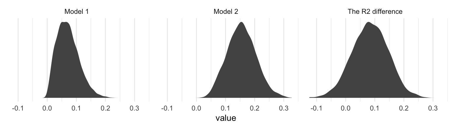
The model coefficient summaries cohere well with those in Table 10.1.
print(model1, digits = 3)## Family: gaussian
## Links: mu = identity; sigma = identity
## Formula: liking ~ 1 + D1 + D2 + sexism
## Data: protest (Number of observations: 129)
## Samples: 4 chains, each with iter = 2000; warmup = 1000; thin = 1;
## total post-warmup samples = 4000
##
## Population-Level Effects:
## Estimate Est.Error l-95% CI u-95% CI Eff.Sample Rhat
## Intercept 4.749 0.619 3.557 5.962 4000 1.000
## D1 0.497 0.233 0.036 0.958 4000 1.000
## D2 0.448 0.227 0.003 0.891 4000 1.000
## sexism 0.110 0.118 -0.118 0.340 4000 1.000
##
## Family Specific Parameters:
## Estimate Est.Error l-95% CI u-95% CI Eff.Sample Rhat
## sigma 1.044 0.067 0.918 1.184 4000 0.999
##
## Samples were drawn using sampling(NUTS). For each parameter, Eff.Sample
## is a crude measure of effective sample size, and Rhat is the potential
## scale reduction factor on split chains (at convergence, Rhat = 1).print(model2, digits = 3)## Family: gaussian
## Links: mu = identity; sigma = identity
## Formula: liking ~ D1 + D2 + sexism + D1:sexism + D2:sexism
## Data: protest (Number of observations: 129)
## Samples: 4 chains, each with iter = 2000; warmup = 1000; thin = 1;
## total post-warmup samples = 4000
##
## Population-Level Effects:
## Estimate Est.Error l-95% CI u-95% CI Eff.Sample Rhat
## Intercept 7.709 1.055 5.721 9.828 1502 1.001
## D1 -4.110 1.522 -7.057 -1.093 1551 1.000
## D2 -3.498 1.429 -6.246 -0.722 1415 1.001
## sexism -0.473 0.206 -0.889 -0.077 1485 1.001
## D1:sexism 0.897 0.291 0.319 1.462 1524 1.001
## D2:sexism 0.778 0.279 0.239 1.318 1406 1.001
##
## Family Specific Parameters:
## Estimate Est.Error l-95% CI u-95% CI Eff.Sample Rhat
## sigma 1.006 0.064 0.890 1.143 2865 1.000
##
## Samples were drawn using sampling(NUTS). For each parameter, Eff.Sample
## is a crude measure of effective sample size, and Rhat is the potential
## scale reduction factor on split chains (at convergence, Rhat = 1).