13.1 Revisiting sexual discrimination in the workplace
Here we load a couple necessary packages, load the data, and take a glimpse().
library(tidyverse)

protest <- read_csv("data/protest/protest.csv")

glimpse(protest)
## Observations: 129
## Variables: 6
## $ subnum <int> 209, 44, 124, 232, 30, 140, 27, 64, 67, 182, 85, 109, 122, 69, 45, 28, 170, 66...
## $ protest <int> 2, 0, 2, 2, 2, 1, 2, 0, 0, 0, 2, 2, 0, 1, 1, 0, 1, 2, 2, 1, 2, 1, 1, 2, 2, 0, ...
## $ sexism <dbl> 4.87, 4.25, 5.00, 5.50, 5.62, 5.75, 5.12, 6.62, 5.75, 4.62, 4.75, 6.12, 4.87, ...
## $ angry <int> 2, 1, 3, 1, 1, 1, 2, 1, 6, 1, 2, 5, 2, 1, 1, 1, 2, 1, 3, 4, 1, 1, 1, 5, 1, 5, ...
## $ liking <dbl> 4.83, 4.50, 5.50, 5.66, 6.16, 6.00, 4.66, 6.50, 1.00, 6.83, 5.00, 5.66, 5.83, ...
## $ respappr <dbl> 4.25, 5.75, 4.75, 7.00, 6.75, 5.50, 5.00, 6.25, 3.00, 5.75, 5.25, 7.00, 4.50, ...With a little ifelse(), we can make the D1 and D2 contrast-coded dummies.
protest <-
  protest %>%
  mutate(D1 = ifelse(protest == 0, -2/3, 1/3),
         D2 = ifelse(protest == 0, 0,
                     ifelse(protest == 1, -1/2, 1/2)))
Load brms.
library(brms)Here are the sub-model formulas.
m_model <- bf(respappr ~ 1 + D1 + D2 + sexism + D1:sexism + D2:sexism)
y_model <- bf(liking   ~ 1 + D1 + D2 + respappr + sexism + D1:sexism + D2:sexism)
Now we’re ready to fit our primary model, the conditional process model with a multicategorical antecedent.
model1 <-
  brm(data = protest, family = gaussian,
      m_model + y_model + set_rescor(FALSE),
      chains = 4, cores = 4)
Here’s the model summary, which coheres reasonably well with the output in Table 13.1.
print(model1, digits = 3)## Family: MV(gaussian, gaussian)
## Links: mu = identity; sigma = identity
## mu = identity; sigma = identity
## Formula: respappr ~ 1 + D1 + D2 + sexism + D1:sexism + D2:sexism
## liking ~ 1 + D1 + D2 + respappr + sexism + D1:sexism + D2:sexism
## Data: protest (Number of observations: 129)
## Samples: 4 chains, each with iter = 2000; warmup = 1000; thin = 1;
## total post-warmup samples = 4000
##
## Population-Level Effects:
## Estimate Est.Error l-95% CI u-95% CI Eff.Sample Rhat
## respappr_Intercept 4.587 0.681 3.239 5.957 4000 0.999
## liking_Intercept 3.478 0.633 2.243 4.705 4000 1.000
## respappr_D1 -2.876 1.443 -5.675 -0.031 3545 1.000
## respappr_D2 1.672 1.622 -1.624 4.845 3595 1.001
## respappr_sexism 0.045 0.132 -0.213 0.312 4000 0.999
## respappr_D1:sexism 0.843 0.280 0.294 1.386 3575 1.000
## respappr_D2:sexism -0.244 0.311 -0.854 0.387 3579 1.001
## liking_D1 -2.690 1.154 -5.001 -0.447 3523 1.000
## liking_D2 0.069 1.334 -2.531 2.632 3310 1.001
## liking_respappr 0.364 0.073 0.220 0.507 4000 1.000
## liking_sexism 0.074 0.104 -0.127 0.273 4000 1.000
## liking_D1:sexism 0.519 0.228 0.074 0.960 3488 1.000
## liking_D2:sexism -0.042 0.255 -0.537 0.457 3358 1.000
##
## Family Specific Parameters:
## Estimate Est.Error l-95% CI u-95% CI Eff.Sample Rhat
## sigma_respappr 1.149 0.075 1.013 1.307 4000 1.001
## sigma_liking 0.917 0.060 0.805 1.041 4000 0.999
##
## Samples were drawn using sampling(NUTS). For each parameter, Eff.Sample
## is a crude measure of effective sample size, and Rhat is the potential
## scale reduction factor on split chains (at convergence, Rhat = 1).The tidybayes::geom_halfeyeh() function gives us a nice way to look at the output with a coefficient plot.
library(tidybayes)

post <- posterior_samples(model1)

post %>%
  select(starts_with("b_")) %>%
  gather() %>%
  mutate(criterion = ifelse(str_detect(key, "respappr"), "criterion: respappr", "criterion: liking"),
         criterion = factor(criterion, levels = c("criterion: respappr", "criterion: liking")),
         key = str_remove(key, "b_respappr_"),
         key = str_remove(key, "b_liking_"),
         key = factor(key, levels = c("Intercept", "respappr", "D2:sexism", "D1:sexism", "sexism", "D2", "D1"))) %>%

  ggplot(aes(x = value, y = key, group = key)) +
  geom_halfeyeh(.prob = c(0.95, 0.5),
                scale = "width", relative_scale = .75,
                color = "white") +
  coord_cartesian(xlim = c(-7, 6)) +
  labs(x = NULL, y = NULL) +
  theme_black() +
  theme(axis.text.y = element_text(hjust = 0),
        axis.ticks.y = element_blank(),
        panel.grid.minor = element_blank(),
        panel.grid.major = element_line(color = "grey20")) +
  facet_wrap(~criterion)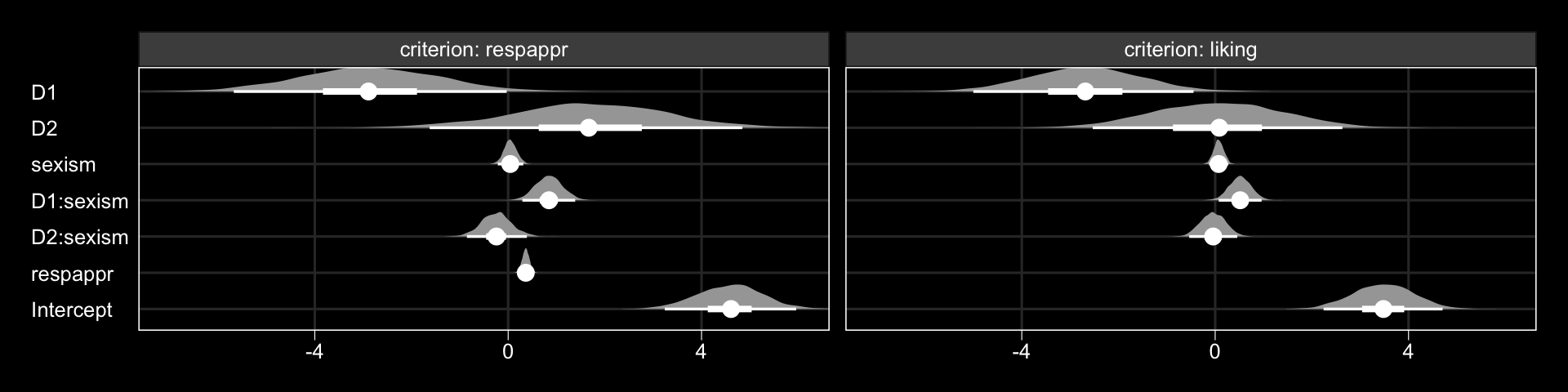
The Bayesian \(R^2\) distributions are reasonably close to the estimates in the text.
bayes_R2(model1) %>% round(digits = 3)## Estimate Est.Error Q2.5 Q97.5
## R2_respappr 0.320 0.052 0.213 0.413
## R2_liking 0.294 0.055 0.181 0.397