3.4 An example with continuous \(X\): Economic stress among small-business owners
Here’s the estress data.
estress <- read_csv("data/estress/estress.csv")

glimpse(estress)
## Observations: 262
## Variables: 7
## $ tenure <dbl> 1.67, 0.58, 0.58, 2.00, 5.00, 9.00, 0.00, 2.50, 0.50, 0.58, 9.00, 1.92, 2.00, 1.42, 0.92...
## $ estress <dbl> 6.0, 5.0, 5.5, 3.0, 4.5, 6.0, 5.5, 3.0, 5.5, 6.0, 5.5, 4.0, 3.0, 2.5, 3.5, 6.0, 4.0, 6.0...
## $ affect <dbl> 2.60, 1.00, 2.40, 1.16, 1.00, 1.50, 1.00, 1.16, 1.33, 3.00, 3.00, 2.00, 1.83, 1.16, 1.16...
## $ withdraw <dbl> 3.00, 1.00, 3.66, 4.66, 4.33, 3.00, 1.00, 1.00, 2.00, 4.00, 4.33, 1.00, 5.00, 1.66, 4.00...
## $ sex <int> 1, 0, 1, 1, 1, 1, 0, 0, 1, 1, 1, 1, 1, 1, 1, 1, 1, 1, 0, 0, 0, 1, 1, 1, 0, 1, 0, 0, 0, 1...
## $ age <int> 51, 45, 42, 50, 48, 48, 51, 47, 40, 43, 57, 36, 33, 29, 33, 48, 40, 45, 37, 42, 54, 57, ...
## $ ese <dbl> 5.33, 6.05, 5.26, 4.35, 4.86, 5.05, 3.66, 6.13, 5.26, 4.00, 2.53, 6.60, 5.20, 5.66, 5.66...The model set up is just like before. There are no complications switching from a binary \(X\) variable to a continuous one.
y_model <- bf(withdraw ~ 1 + estress + affect)
m_model <- bf(affect ~ 1 + estress)
With our y_model and m_model defined, we’re ready to fit.
model2 <-
  brm(data = estress, family = gaussian,
      y_model + m_model + set_rescor(FALSE),
      chains = 4, cores = 4)
Let’s take a look.
print(model2, digits = 3)## Family: MV(gaussian, gaussian)
## Links: mu = identity; sigma = identity
## mu = identity; sigma = identity
## Formula: withdraw ~ 1 + estress + affect
## affect ~ 1 + estress
## Data: estress (Number of observations: 262)
## Samples: 4 chains, each with iter = 2000; warmup = 1000; thin = 1;
## total post-warmup samples = 4000
##
## Population-Level Effects:
## Estimate Est.Error l-95% CI u-95% CI Eff.Sample Rhat
## withdraw_Intercept 1.450 0.257 0.939 1.953 4000 1.000
## affect_Intercept 0.800 0.145 0.523 1.080 4000 0.999
## withdraw_estress -0.077 0.053 -0.181 0.025 4000 1.000
## withdraw_affect 0.766 0.104 0.561 0.969 4000 1.000
## affect_estress 0.173 0.030 0.113 0.230 4000 0.999
##
## Family Specific Parameters:
## Estimate Est.Error l-95% CI u-95% CI Eff.Sample Rhat
## sigma_withdraw 1.139 0.048 1.048 1.232 4000 0.999
## sigma_affect 0.686 0.031 0.628 0.750 4000 1.000
##
## Samples were drawn using sampling(NUTS). For each parameter, Eff.Sample
## is a crude measure of effective sample size, and Rhat is the potential
## scale reduction factor on split chains (at convergence, Rhat = 1).The ‘Eff.Sample’ and ‘Rhat’ values look great. Happily, the values in our summary cohere well with those Hayes reported in Table 3.5. Here are our \(R^2\) values.
bayes_R2(model2)## Estimate Est.Error Q2.5 Q97.5
## R2_withdraw 0.1815384 0.03849542 0.1044912 0.2572579
## R2_affect 0.1169312 0.03505706 0.0524473 0.1861113These are also quite similar to those in the text. Here’s our indirect effect.
# putting the posterior draws into a data frame
post <- posterior_samples(model2)

# computing the ab coefficient with multiplication
post <-
  post %>%
  mutate(ab = b_affect_estress*b_withdraw_affect)

# getting the posterior median and 95% intervals with `quantile()`
quantile(post$ab, probs = c(.5, .025, .975)) %>% round(digits = 3)
## 50% 2.5% 97.5%
## 0.131 0.079 0.195We can visualize its shape, median, and 95% intervals in a density plot.
post %>%
  ggplot(aes(x = ab)) +
  geom_density(color = "transparent",
               fill = colorblind_pal()(7)[7]) +
  geom_vline(xintercept = quantile(post$ab, probs = c(.025, .5, .975)),
             color = "white", linetype = c(2, 1, 2), size = c(.5, .8, .5)) +
  scale_x_continuous(breaks = quantile(post$ab, probs = c(.025, .5, .975)),
                     labels = quantile(post$ab, probs = c(.025, .5, .975)) %>% round(2) %>% as.character()) +
  scale_y_continuous(NULL, breaks = NULL) +
  labs(title = expression(paste("Behold our ", italic("ab"), "!")),
       x = NULL) +
  theme_classic()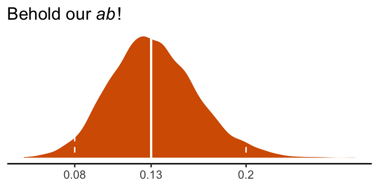
Here’s \(c'\), the direct effect of esterss predicting withdraw.
posterior_summary(model2)["b_withdraw_estress", ]## Estimate Est.Error Q2.5 Q97.5
## -0.07663292 0.05256371 -0.18050458 0.02503829It has wide flapping intervals which do straddle zero. A little addition will give us the direct effect, \(c\).
post <-
  post %>%
  mutate(c = b_withdraw_estress + ab)

quantile(post$c, probs = c(.5, .025, .975)) %>% round(digits = 3)
## 50% 2.5% 97.5%
## 0.056 -0.053 0.165