7.6 Artificial categorization and subgroups

There are multiple ways to dichotomize the data by skeptic. A quick simple way is to use ifelse() to make a skeptic_hi dummy.

disaster <-
  disaster %>% 
  mutate(skeptic_hi = ifelse(skeptic >= mean(skeptic), 1, 0))

With our dummy in hand, we’re ready to fit the two models.

model6_low <-
  brm(data = disaster %>% filter(skeptic_hi == 0), 
      family = gaussian,
      justify ~ 1 + frame,
      chains = 4, cores = 4)

model6_high <-
  update(model6_low, newdata = disaster %>% filter(skeptic_hi == 1),
         chains = 4, cores = 4)

The coefficient summaries:

fixef(model6_low) %>% round(digits = 3)

##           Estimate Est.Error   Q2.5 Q97.5
## Intercept    2.626     0.099  2.431 2.824
## frame       -0.108     0.145 -0.390 0.173

fixef(model6_high) %>% round(digits = 3)

##           Estimate Est.Error  Q2.5 Q97.5
## Intercept    3.070     0.144 2.786 3.348
## frame        0.477     0.209 0.071 0.891

You can use fitted() to get the posterior means and other summaries for the two frame groups, by model.

fitted(model6_low, 
       newdata = tibble(frame = 0:1)) %>% 
  round(digits = 3)

##      Estimate Est.Error  Q2.5 Q97.5
## [1,]    2.626     0.099 2.431 2.824
## [2,]    2.518     0.105 2.309 2.724

fitted(model6_high, 
       newdata = tibble(frame = 0:1)) %>% 
  round(digits = 3)

##      Estimate Est.Error  Q2.5 Q97.5
## [1,]    3.070     0.144 2.786 3.348
## [2,]    3.548     0.149 3.256 3.836

Do note that though brms ‘Est.Error’ is the posterior \(SD\) for the coefficient, it is not the same thing as descriptive statistic \(SD\) of a subset of the data. Thus, although our ‘Estimates’ correspond nicely to the mean values Hayes reported in the middle of page 264, his \(SD\)s will not match up with our ‘Est.Error’ values, and nor should they.

Anyway, our results don’t yield \(t\)-tests. But you don’t need those anyway. We’re working within the regression paradigm! But if you’re really interested in the sub-model-implied differences between the two levels of frame by skeptic_hi subgroup, all you need is the frame coefficient of model6_low and model6_high. Here we’ll use bind_rows() to combine their posterior samples and then plot.

posterior_samples(model6_low) %>% 
  select(b_frame) %>% 
  bind_rows(
    posterior_samples(model6_high) %>%
      select(b_frame)
  ) %>% 
  mutate(model = rep(c("model6_low", "model6_high"), each = 4000)) %>% 
    
  ggplot(aes(x = b_frame, fill = model)) +
  geom_density(size = 0, alpha = .8) +
  scale_fill_manual(NULL, 
                    values = dutchmasters$little_street[c(1, 9)] %>% as.character()) +
  scale_y_continuous(NULL, breaks = NULL) +
  labs(subtitle = "The difference score distributions between frame levels,\ncolor coded by mean-split skeptic",
       x = NULL) +
  theme_07

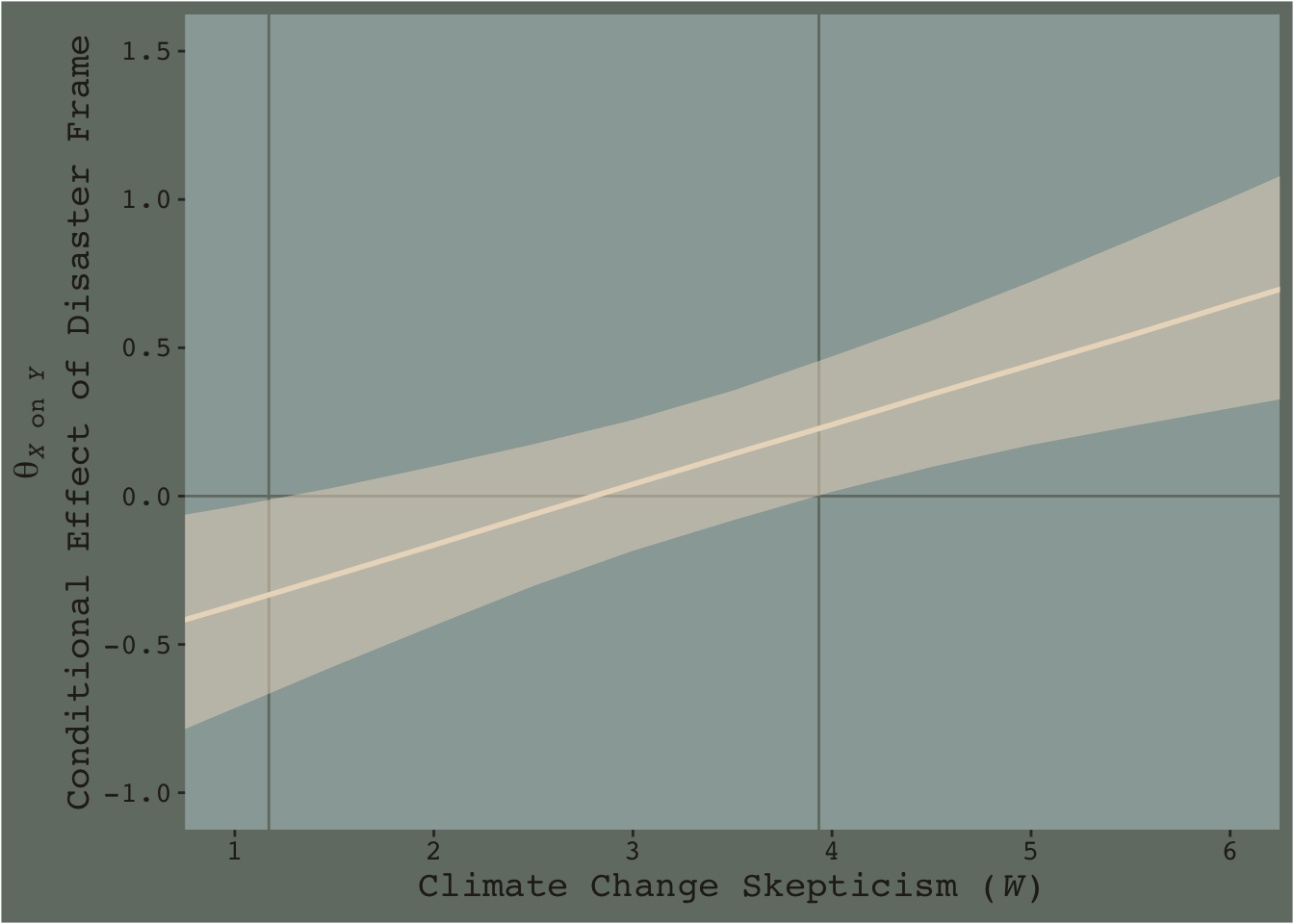
As within the frequentist paradigm, please don’t mean split as a Bayesian. When possible, use all available data and use the regression formula to model theoretically-meaningful variables in your analyses.