8.3 Hierarchical versus simultaneous entry

Here’s our multivariable but non-moderation model, model4.

model4 <-
  update(model1, 
         formula = justify ~ 1 + skeptic + frame,
         chains = 4, cores = 4)

Here we’ll compute the corresponding \(R^2\) and compare it with the one for the original interaction model with a difference score.

# the moderation model's R2
R2s <-
  bayes_R2(model1, summary = F) %>% 
  as_tibble() %>% 
  rename(moderation_model = R2) %>% 
  # here we add the multivaraible model's R2
  bind_cols(
    bayes_R2(model4, summary = F) %>% 
      as_tibble() %>% 
      rename(multivariable_model = R2)
  ) %>% 
  # we'll need a difference score
  mutate(difference = moderation_model - multivariable_model) %>% 
  # putting the data in the long format and grouping will make summarizing easier
  gather(R2, value)

R2s %>% 
  group_by(R2) %>% 
  summarize(median = median(value),
            ll = quantile(value, probs = .025),
            ul = quantile(value, probs = .975)) %>% 
  mutate_if(is.double, round, digits = 3)

## # A tibble: 3 x 4
##   R2                  median     ll    ul
##   <chr>                <dbl>  <dbl> <dbl>
## 1 difference           0.05  -0.074 0.169
## 2 moderation_model     0.249  0.16  0.335
## 3 multivariable_model  0.2    0.111 0.286

Note that the Bayesian \(R^2\) performed differently than the \(F\)-test in the text.

R2s %>% 
  filter(R2 == "difference") %>% 

  ggplot(aes(x = value)) +
  geom_density(aes(fill = model), size = 0, fill = ochre_palettes[["olsen_seq"]][14]) +
  scale_y_continuous(NULL, breaks = NULL) +
  labs(title = expression(paste("The Bayesian ", Delta, italic(R)^2, " distribution")),
       subtitle = "Although most of the posterior mass is positive--suggesting the moderation model accounted for more variance than\nthe simple multivariable model--, a substantial portion of the postrior is within the negative parameter space. Sure,\nif we had to bet, the safer bet is on the moderation model. But that bet wouled be quite uncertain and we might well\nloose our shirts. Also, note the width of the distribution; credible values range from -0.1 to nearly 0.2.",
       x = NULL) +
  coord_cartesian(xlim = c(-.4, .4)) +
  theme_08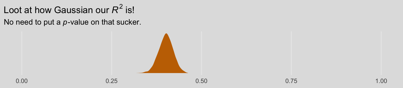

We can also compare these with the LOO, which, as is typical of information criteria, corrects for model coplexity.

(l_model1 <- loo(model1))

## 
## Computed from 4000 by 211 log-likelihood matrix
## 
##          Estimate   SE
## elpd_loo   -259.2 10.8
## p_loo         5.6  0.9
## looic       518.4 21.6
## ------
## Monte Carlo SE of elpd_loo is 0.0.
## 
## All Pareto k estimates are good (k < 0.5).
## See help('pareto-k-diagnostic') for details.

(l_model4 <- loo(model4))

## 
## Computed from 4000 by 211 log-likelihood matrix
## 
##          Estimate   SE
## elpd_loo   -264.6 11.2
## p_loo         4.6  0.9
## looic       529.3 22.4
## ------
## Monte Carlo SE of elpd_loo is 0.0.
## 
## All Pareto k estimates are good (k < 0.5).
## See help('pareto-k-diagnostic') for details.

The LOO values aren’t of interest in and of themselves. However, the bottom of the loo() output was useful because for both models we learned that “All Pareto k estimates are good (k < 0.5).”, which assures us that we didn’t have a problem with overly-influential outlier values. But even though the LOO values weren’t interesting themselves, their difference score is. We’ll use compare_ic() to get that.

compare_ic(l_model1, l_model4)

##                  LOOIC    SE
## model1          518.39 21.61
## model4          529.26 22.37
## model1 - model4 -10.87  8.16

As a reminder, we generally prefer models with lower information criteria, which in this case is clearly the moderation model (i.e., model1). However, the standard error value for the difference is quite large, which suggests that the model with the lowest value isn’t the clear winner. Happily, these results match nicely with the Bayesian \(R^2\) difference score. The moderation model appears somewhat better than the multivariable model, but its superiority is hardly decisive.