4.2 Confounding and causal order
4.2.1 Accounting for confounding and epiphenomenal association.
Here we load a couple necessary packages, load the data, and take a peek at them.
library(tidyverse)

estress <- read_csv("data/estress/estress.csv")

glimpse(estress)
## Observations: 262
## Variables: 7
## $ tenure <dbl> 1.67, 0.58, 0.58, 2.00, 5.00, 9.00, 0.00, 2.50, 0.50, 0.58, 9.00, 1.92, 2.00, 1.42, 0.92...
## $ estress <dbl> 6.0, 5.0, 5.5, 3.0, 4.5, 6.0, 5.5, 3.0, 5.5, 6.0, 5.5, 4.0, 3.0, 2.5, 3.5, 6.0, 4.0, 6.0...
## $ affect <dbl> 2.60, 1.00, 2.40, 1.16, 1.00, 1.50, 1.00, 1.16, 1.33, 3.00, 3.00, 2.00, 1.83, 1.16, 1.16...
## $ withdraw <dbl> 3.00, 1.00, 3.66, 4.66, 4.33, 3.00, 1.00, 1.00, 2.00, 4.00, 4.33, 1.00, 5.00, 1.66, 4.00...
## $ sex <int> 1, 0, 1, 1, 1, 1, 0, 0, 1, 1, 1, 1, 1, 1, 1, 1, 1, 1, 0, 0, 0, 1, 1, 1, 0, 1, 0, 0, 0, 1...
## $ age <int> 51, 45, 42, 50, 48, 48, 51, 47, 40, 43, 57, 36, 33, 29, 33, 48, 40, 45, 37, 42, 54, 57, ...
## $ ese <dbl> 5.33, 6.05, 5.26, 4.35, 4.86, 5.05, 3.66, 6.13, 5.26, 4.00, 2.53, 6.60, 5.20, 5.66, 5.66...The lowerCor() function from the psych package makes it easy to estimate the lower triangle of a correlation matrix.
psych::lowerCor(estress, digits = 3)## tenure estrss affect wthdrw sex age ese
## tenure 1.000
## estress 0.068 1.000
## affect -0.065 0.340 1.000
## withdraw -0.035 0.064 0.417 1.000
## sex -0.003 0.133 0.046 0.050 1.000
## age 0.266 0.066 -0.018 -0.035 0.083 1.000
## ese -0.060 -0.158 -0.246 -0.243 0.028 -0.083 1.000Let’s open brms.
library(brms)Recall that if you want the correlations with Bayesian estimation and those sweet Bayesian credible intervals, you set up an intercept-only multivariate model.
model1 <-
  brm(data = estress, family = gaussian,
      cbind(ese, estress, affect, withdraw) ~ 1,
      chains = 4, cores = 4)
The summary:
print(model1, digits = 3)## Family: MV(gaussian, gaussian, gaussian, gaussian)
## Links: mu = identity; sigma = identity
## mu = identity; sigma = identity
## mu = identity; sigma = identity
## mu = identity; sigma = identity
## Formula: ese ~ 1
## estress ~ 1
## affect ~ 1
## withdraw ~ 1
## Data: estress (Number of observations: 262)
## Samples: 4 chains, each with iter = 2000; warmup = 1000; thin = 1;
## total post-warmup samples = 4000
##
## Population-Level Effects:
## Estimate Est.Error l-95% CI u-95% CI Eff.Sample Rhat
## ese_Intercept 5.607 0.061 5.485 5.725 4000 1.001
## estress_Intercept 4.620 0.092 4.440 4.796 4000 1.000
## affect_Intercept 1.598 0.045 1.508 1.687 4000 1.001
## withdraw_Intercept 2.322 0.078 2.174 2.476 4000 0.999
##
## Family Specific Parameters:
## Estimate Est.Error l-95% CI u-95% CI Eff.Sample Rhat
## sigma_ese 0.954 0.043 0.873 1.044 4000 1.000
## sigma_estress 1.437 0.064 1.317 1.568 4000 0.999
## sigma_affect 0.730 0.032 0.668 0.799 4000 0.999
## sigma_withdraw 1.257 0.055 1.151 1.370 4000 0.999
##
## Residual Correlations:
## Estimate Est.Error l-95% CI u-95% CI Eff.Sample Rhat
## rescor(ese,estress) -0.154 0.061 -0.272 -0.033 4000 1.000
## rescor(ese,affect) -0.239 0.059 -0.352 -0.120 4000 0.999
## rescor(estress,affect) 0.335 0.055 0.228 0.439 4000 1.000
## rescor(ese,withdraw) -0.237 0.058 -0.347 -0.121 4000 1.000
## rescor(estress,withdraw) 0.061 0.061 -0.059 0.181 4000 0.999
## rescor(affect,withdraw) 0.410 0.052 0.306 0.509 4000 1.000
##
## Samples were drawn using sampling(NUTS). For each parameter, Eff.Sample
## is a crude measure of effective sample size, and Rhat is the potential
## scale reduction factor on split chains (at convergence, Rhat = 1).Since we have posteriors for the correlations, why not plot them? Here we use the theme_black() from brms and a color scheme from the viridis package.
library(viridis)

posterior_samples(model1) %>%
  select(rescor__ese__estress, rescor__ese__affect, rescor__estress__withdraw) %>%
  gather() %>%

  ggplot(aes(x = value, fill = key)) +
  geom_density(alpha = .85, color = "transparent") +
  scale_fill_viridis(discrete = T, option = "D", direction = -1,
                     labels = c(expression(paste(rho["ese, affect"])),
                                expression(paste(rho["ese, estress"])),
                                expression(paste(rho["estress, withdraw"]))),
                     guide = guide_legend(label.hjust = 0,
                                          label.theme = element_text(size = 15, angle = 0, color = "white"),
                                          title.theme = element_blank())) +
  coord_cartesian(xlim = c(-1, 1)) +
  labs(title = "Our correlation density plot",
       x = NULL) +
  theme_black() +
  theme(panel.grid = element_blank(),
        axis.text.y = element_text(hjust = 0),
        axis.ticks.y = element_blank())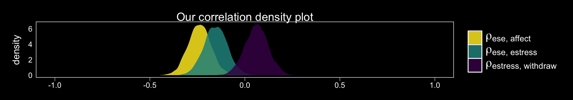
Before we fit our mediation model with brm(), we’ll specify the sub-models, here.
y_model <- bf(withdraw ~ 1 + estress + affect + ese + sex + tenure)
m_model <- bf(affect ~ 1 + estress + ese + sex + tenure)
With y_model and m_model defined, we’re ready to fit.
model2 <-
  brm(data = estress, family = gaussian,
      y_model + m_model + set_rescor(FALSE),
      chains = 4, cores = 4)
Here’s the summary:
print(model2, digits = 3)## Family: MV(gaussian, gaussian)
## Links: mu = identity; sigma = identity
## mu = identity; sigma = identity
## Formula: withdraw ~ 1 + estress + affect + ese + sex + tenure
## affect ~ 1 + estress + ese + sex + tenure
## Data: estress (Number of observations: 262)
## Samples: 4 chains, each with iter = 2000; warmup = 1000; thin = 1;
## total post-warmup samples = 4000
##
## Population-Level Effects:
## Estimate Est.Error l-95% CI u-95% CI Eff.Sample Rhat
## withdraw_Intercept 2.751 0.554 1.663 3.823 4000 0.999
## affect_Intercept 1.784 0.308 1.189 2.375 4000 0.999
## withdraw_estress -0.093 0.052 -0.194 0.012 4000 1.000
## withdraw_affect 0.708 0.105 0.508 0.912 4000 1.000
## withdraw_ese -0.213 0.077 -0.366 -0.064 4000 0.999
## withdraw_sex 0.126 0.143 -0.153 0.402 4000 0.999
## withdraw_tenure -0.002 0.011 -0.024 0.019 4000 1.000
## affect_estress 0.160 0.030 0.102 0.219 4000 0.999
## affect_ese -0.155 0.045 -0.243 -0.069 4000 0.999
## affect_sex 0.016 0.088 -0.159 0.190 4000 0.999
## affect_tenure -0.011 0.006 -0.023 0.001 4000 0.999
##
## Family Specific Parameters:
## Estimate Est.Error l-95% CI u-95% CI Eff.Sample Rhat
## sigma_withdraw 1.127 0.049 1.036 1.229 4000 1.000
## sigma_affect 0.671 0.031 0.614 0.735 4000 1.000
##
## Samples were drawn using sampling(NUTS). For each parameter, Eff.Sample
## is a crude measure of effective sample size, and Rhat is the potential
## scale reduction factor on split chains (at convergence, Rhat = 1).In the printout, notice how first within intercepts and then with covariates and sigma, the coefficients are presented as for withdraw first and then affect. Also notice how the coefficients for the covariates are presented in the same order for each criterions. Hopefully that’ll make it easier to sift through the printout. Happily, our coefficients are quite similar to those in Table 4.1.
Here are the \(R^2\) values.
bayes_R2(model2) %>% round(digits = 3)## Estimate Est.Error Q2.5 Q97.5
## R2_withdraw 0.213 0.039 0.138 0.287
## R2_affect 0.171 0.038 0.099 0.245These are also in the same ballpark, but a little higher. Why not glance at their densities?
bayes_R2(model2, summary = F) %>%
  as_tibble() %>%
  gather() %>%

  ggplot(aes(x = value, fill = key)) +
  geom_density(color = "transparent", alpha = .85) +
  scale_fill_manual(values = c(viridis_pal(option = "A")(7)[c(7, 3)]),
                    labels = c("affect", "withdraw"),
                    guide = guide_legend(title.theme = element_blank())) +
  scale_y_continuous(NULL, breaks = NULL) +
  coord_cartesian(xlim = 0:1) +
  labs(title = expression(paste("The ", italic("R")^{2}, " distributions for model2")),
       x = NULL) +
  theme_black() +
  theme(panel.grid = element_blank())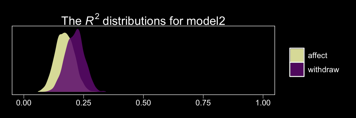
Here we retrieve the posterior samples, compute the indirect effect, and summarize the indirect effect with quantile().
post <-
  posterior_samples(model2) %>%
  mutate(ab = b_affect_estress*b_withdraw_affect)

quantile(post$ab, probs = c(.5, .025, .975)) %>%
  round(digits = 3)
## 50% 2.5% 97.5%
## 0.112 0.064 0.171The results are similar to those in the text (p. 127). Here’s what it looks like.
post %>%

  ggplot(aes(x = ab)) +
  geom_density(color = "transparent",
               fill = viridis_pal(option = "A")(7)[5]) +
  geom_vline(xintercept = quantile(post$ab, probs = c(.5, .025, .975)),
             color = "black", linetype = c(1, 3, 3)) +
  scale_y_continuous(NULL, breaks = NULL) +
  xlab(expression(italic("ab"))) +
  theme_black() +
  theme(panel.grid = element_blank())
Once again, those sweet Bayesian credible intervals get the job done.
Here’s a way to get both the direct effect, \(c'\) (i.e., b_withdraw_estress), and the total effect, \(c\) (i.e., \(c'\) + \(ab\)) of estress on withdraw.
post %>%
  mutate(c = b_withdraw_estress + ab) %>%
  rename(c_prime = b_withdraw_estress) %>%
  select(c_prime, c) %>%
  gather() %>%
  group_by(key) %>%
  summarize(mean = mean(value),
            ll = quantile(value, probs = .025),
            ul = quantile(value, probs = .975)) %>%
  mutate_if(is_double, round, digits = 3)
## # A tibble: 2 x 4
## key mean ll ul
## <chr> <dbl> <dbl> <dbl>
## 1 c 0.02 -0.086 0.13
## 2 c_prime -0.093 -0.194 0.012Both appear pretty small. Which leads us to the next section…