5.3 Statistical inference
5.3.1 Inference about the direct and total effects.
We’re not going to bother with \(p\)-values and we’ve already computed the 95% Bayesian credible intervals, above. But we can examine our parameters with a density plot.
post %>%
  select(c, c_prime) %>%
  gather() %>%

  ggplot(aes(x = value, fill = key, color = key)) +
  geom_vline(xintercept = 0, color = "black") +
  geom_density(alpha = .5) +
  scale_color_ptol(NULL) +
  scale_fill_ptol(NULL) +
  scale_y_continuous(NULL, breaks = NULL) +
  labs(title = expression(paste("It appears zero is more credible for the direct effect, ", italic(c), "', than it is the total effect, ", italic(c), ".")),
       x = NULL) +
  coord_cartesian(xlim = -c(-1.5, 1.5)) +
  theme_minimal()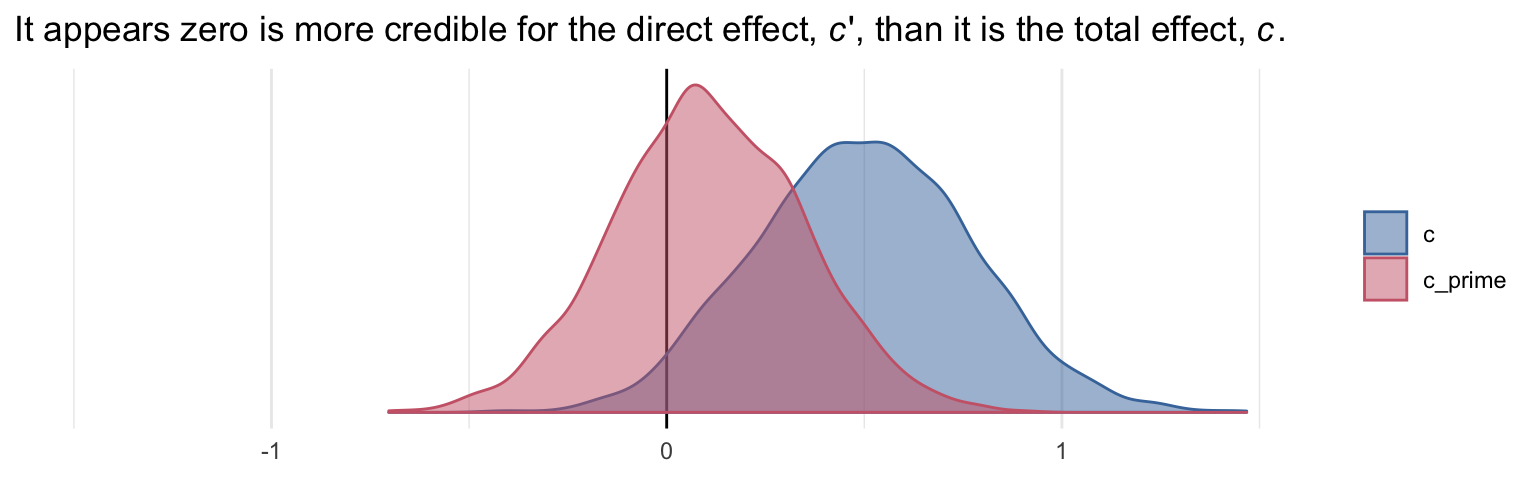
5.3.2 Inference about specific indirect effects.
Again, no need to worry about bootstrapping within the Bayesian paradigm. We can compute high-quality percentile-based intervals with our HMC-based posterior samples.
post %>%
  select(a1b1, a2b2) %>%
  gather() %>%
  group_by(key) %>%
  summarize(ll = quantile(value, probs = .025),
            ul = quantile(value, probs = .975)) %>%
  mutate_if(is.double, round, digits = 3)
## # A tibble: 2 x 3
## key ll ul
## <chr> <dbl> <dbl>
## 1 a1b1 0.011 0.445
## 2 a2b2 0.003 0.4235.3.3 Pairwise comparisons between specific indirect effects.
Within the Bayesian paradigm, it’s straightforward to compare indirect effects. All one has to do is compute a difference score and summarize it somehow. Here it is, a1b1 minus a2b2.
post <-
  post %>%
  mutate(difference = a1b1 - a2b2)

post %>%
  summarize(mean = mean(difference),
            ll = quantile(difference, probs = .025),
            ul = quantile(difference, probs = .975)) %>%
  mutate_if(is.double, round, digits = 3)
## mean ll ul
## 1 0.014 -0.3 0.331Why not plot?
post %>%

  ggplot(aes(x = difference)) +
  geom_vline(xintercept = 0, color = "black", linetype = 2) +
  geom_density(color = "black", fill = "black", alpha = .5) +
  scale_y_continuous(NULL, breaks = NULL) +
  labs(title = "The difference score between the indirect effects",
       subtitle = expression(paste("No ", italic(p), "-value or 95% intervals needed for this one.")),
       x = NULL) +
  coord_cartesian(xlim = -1:1) +
  theme_minimal()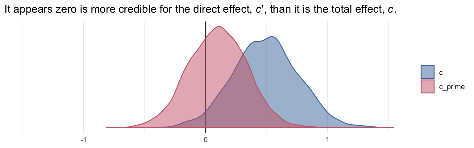
Although note well that this does not mean their difference is exactly zero. The shape of the posterior distribution testifies our uncertainty in their difference. Our best bet is that the difference is approximately zero, but it could easily be plus or minus a quarter of a point or more.
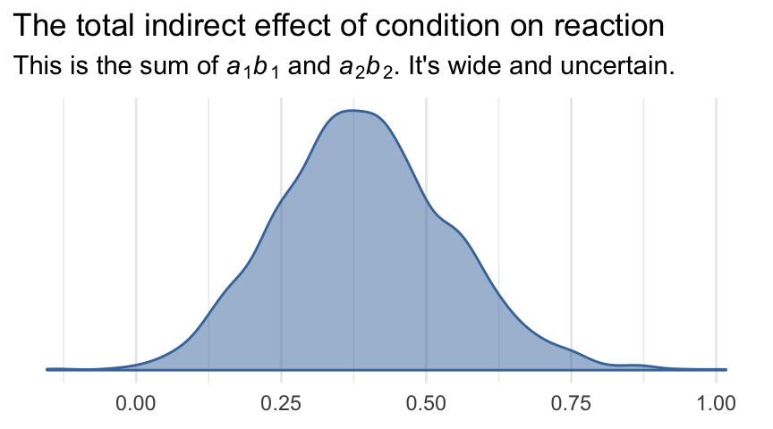
5.3.4 Inference about the total indirect effect.
Here’s the plot.
post %>%

  ggplot(aes(x = total_indirect_effect, fill = factor(0), color = factor(0))) +
  geom_density(alpha = .5) +
  scale_color_ptol() +
  scale_fill_ptol() +
  scale_y_continuous(NULL, breaks = NULL) +
  labs(title = "The total indirect effect of condition on reaction",
       subtitle = expression(paste("This is the sum of ", italic(a)[1], italic(b)[1], " and ", italic(a)[2], italic(b)[2], ". It's wide and uncertain.")),
       x = NULL) +
  theme_minimal() +
  theme(legend.position = "none")