4.3 Effect size
4.3.1 The partially standardized effect.
We get \(SD\)s using the sd() function. Here’s the \(SD\) for our \(Y\) variable, withdraw.
sd(estress$withdraw)## [1] 1.24687Here we compute the partially standardized effect sizes for \(c'\) and \(ab\) by dividing those vectors in our post object by sd(estress$withdraw), which we saved as SD_y.
SD_y <- sd(estress$withdraw)

post %>%
  mutate(c_prime_ps = b_withdraw_estress/SD_y,
         ab_ps = ab/SD_y) %>%
  mutate(c_ps = c_prime_ps + ab_ps) %>%
  select(c_prime_ps, ab_ps, c_ps) %>%
  gather() %>%
  group_by(key) %>%
  summarize(mean = mean(value),
            median = median(value),
            ll = quantile(value, probs = .025),
            ul = quantile(value, probs = .975)) %>%
  mutate_if(is_double, round, digits = 3)
## # A tibble: 3 x 5
## key mean median ll ul
## <chr> <dbl> <dbl> <dbl> <dbl>
## 1 ab_ps 0.091 0.089 0.051 0.137
## 2 c_prime_ps -0.075 -0.075 -0.155 0.01
## 3 c_ps 0.016 0.015 -0.069 0.104The results are similar, though not identical, to those in the text. Here we have both rounding error and estimation differences at play. The plots:
post %>%
  mutate(c_prime_ps = b_withdraw_estress/SD_y,
         ab_ps = ab/SD_y) %>%
  mutate(c_ps = c_prime_ps + ab_ps) %>%
  select(c_prime_ps, ab_ps, c_ps) %>%
  gather() %>%

  ggplot(aes(x = value, fill = key)) +
  geom_density(alpha = .85, color = "transparent") +
  scale_fill_viridis(discrete = T, option = "D") +
  scale_y_continuous(NULL, breaks = NULL) +
  labs(title = "Partially-standardized coefficients",
       x = NULL) +
  theme_black() +
  theme(panel.grid = element_blank(),
        legend.position = "none") +
  facet_wrap(~key, ncol = 3)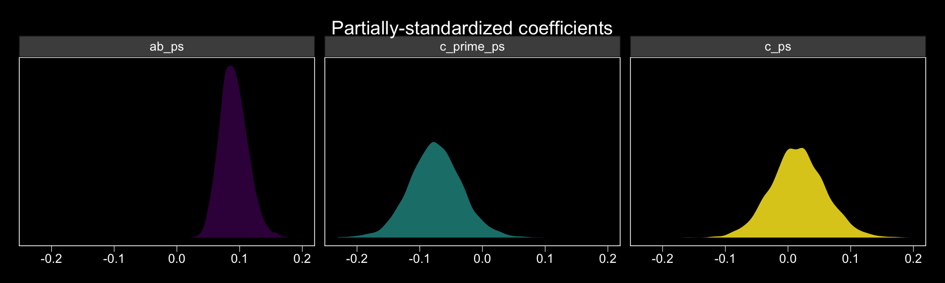
On page 135, Hayes revisited the model from section 3.3. We’ll have to reload the data and refit that model to follow along.
pmi <- read_csv("data/pmi/pmi.csv")

y_model <- bf(reaction ~ 1 + pmi + cond)
m_model <- bf(pmi ~ 1 + cond)
model3 <-
brm(data = pmi, family = gaussian,
y_model + m_model + set_rescor(FALSE),
chains = 4, cores = 4)The partially-standardized parameters require some posterior_samples() wrangling.
post <- posterior_samples(model3)

SD_y <- sd(pmi$reaction)

post %>%
  mutate(ab = b_pmi_cond * b_reaction_pmi,
         c_prime = b_reaction_cond) %>%
  mutate(ab_ps = ab/SD_y,
         c_prime_ps = c_prime/SD_y) %>%
  mutate(c_ps = c_prime_ps + ab_ps) %>%
  select(c_prime_ps, ab_ps, c_ps) %>%
  gather() %>%
  group_by(key) %>%
  summarize(mean = mean(value),
            median = median(value),
            ll = quantile(value, probs = .025),
            ul = quantile(value, probs = .975)) %>%
  mutate_if(is_double, round, digits = 3)
## # A tibble: 3 x 5
## key mean median ll ul
## <chr> <dbl> <dbl> <dbl> <dbl>
## 1 ab_ps 0.154 0.149 0.006 0.327
## 2 c_prime_ps 0.16 0.162 -0.176 0.484
## 3 c_ps 0.314 0.315 -0.047 0.667Happily, these results are closer to those in the text than with the previous example.
4.3.2 The completely standardized effect.
Note. Hayes could have made this clearer in the text, but the estress model he referred to in this section was the one from way back in section 3.5, not the one from earlier in this chapter.
One way to get a standardized solution is to standardize the variables in the data and then fit the model with those standardized variables. To do so, we’ll revisit our custom standardize(), put it to work, and fit the standardized version of the model from section 3.5, which we’ll call model4.With our y_model and m_model defined, we’re ready to fit.
sandardize <- function(x){
  (x - mean(x))/sd(x)
}

estress <-
  estress %>%
  mutate(withdraw_z = sandardize(withdraw),
         estress_z  = sandardize(estress),
         affect_z   = sandardize(affect))

y_model <- bf(withdraw_z ~ 1 + estress_z + affect_z)
m_model <- bf(affect_z ~ 1 + estress_z)
model4 <-
brm(data = estress, family = gaussian,
y_model + m_model + set_rescor(FALSE),
chains = 4, cores = 4)Here they are, our newly standardized coefficients:
fixef(model4) %>% round(digits = 3)## Estimate Est.Error Q2.5 Q97.5
## withdrawz_Intercept -0.001 0.056 -0.111 0.109
## affectz_Intercept -0.002 0.058 -0.112 0.111
## withdrawz_estress_z -0.089 0.061 -0.210 0.034
## withdrawz_affect_z 0.448 0.062 0.328 0.571
## affectz_estress_z 0.340 0.060 0.222 0.458Here we do the wrangling necessary to spell out the standardized effects for \(ab\), \(c'\), and \(c\).
post <- posterior_samples(model4)

post %>%
  mutate(ab_s = b_affectz_estress_z * b_withdrawz_affect_z,
         c_prime_s = b_withdrawz_estress_z) %>%
  mutate(c_s = ab_s + c_prime_s) %>%
  select(c_prime_s, ab_s, c_s) %>%
  gather() %>%
  group_by(key) %>%
  summarize(mean = mean(value),
            median = median(value),
            ll = quantile(value, probs = .025),
            ul = quantile(value, probs = .975)) %>%
  mutate_if(is_double, round, digits = 3)
## # A tibble: 3 x 5
## key mean median ll ul
## <chr> <dbl> <dbl> <dbl> <dbl>
## 1 ab_s 0.152 0.151 0.091 0.223
## 2 c_prime_s -0.089 -0.09 -0.21 0.034
## 3 c_s 0.063 0.064 -0.066 0.189Let’s confirm that we can recover these values by applying the formulas on page 135 to the unstandardized model, which we’ll call model5. First, we’ll have to fit that model since we haven’t fit that one since Chapter 3.
y_model <- bf(withdraw ~ 1 + estress + affect)
m_model <- bf(affect ~ 1 + estress)

model5 <-
  brm(data = estress, family = gaussian,
      y_model + m_model + set_rescor(FALSE),
      chains = 4, cores = 4)
Here are the unstandardized coefficients:
fixef(model5) %>% round(digits = 3)## Estimate Est.Error Q2.5 Q97.5
## withdraw_Intercept 1.444 0.257 0.929 1.949
## affect_Intercept 0.797 0.140 0.527 1.083
## withdraw_estress -0.077 0.053 -0.179 0.026
## withdraw_affect 0.771 0.105 0.565 0.978
## affect_estress 0.173 0.029 0.114 0.230On pages 135–136, Hayes provided the formulas to compute the standardized effects:
\[c'_{cs} = \frac{SD_X(c')}{SD_{Y}} = SD_{X}(c'_{ps})\]
\[ab_{cs} = \frac{SD_X(ab)}{SD_{Y}} = SD_{X}(ab_{ps})\]
\[c_{cs} = \frac{SD_X(c)}{SD_{Y}} = c'_{cs} + ab_{ps}\]
Here we put them in action to standardize the unstandardized results.
post <- posterior_samples(model5)

SD_x <- sd(estress$estress)
SD_y <- sd(estress$withdraw)

post %>%
  mutate(ab = b_affect_estress * b_withdraw_affect,
         c_prime = b_withdraw_estress) %>%
  mutate(ab_s = (SD_x*ab)/SD_y,
         c_prime_s = (SD_x*c_prime)/SD_y) %>%
  mutate(c_s = ab_s + c_prime_s) %>%
  select(c_prime_s, ab_s, c_s) %>%
  gather() %>%
  group_by(key) %>%
  summarize(mean = mean(value),
            median = median(value),
            ll = quantile(value, probs = .025),
            ul = quantile(value, probs = .975)) %>%
  mutate_if(is_double, round, digits = 3)
## # A tibble: 3 x 5
## key mean median ll ul
## <chr> <dbl> <dbl> <dbl> <dbl>
## 1 ab_s 0.153 0.151 0.092 0.22
## 2 c_prime_s -0.088 -0.087 -0.205 0.03
## 3 c_s 0.065 0.065 -0.062 0.188Success!
4.3.3 Some (problematic) measures only for indirect effects.
Hayes recommended against these, so I’m not going to bother working any examples.