8.1 Moderation with a dichotomous moderator
Here we load a couple necessary packages, load the data, and take a glimpse().
library(tidyverse)
library(brms)

disaster <- read_csv("data/disaster/disaster.csv")

glimpse(disaster)
## Observations: 211
## Variables: 5
## $ id <int> 1, 2, 3, 4, 5, 6, 7, 8, 9, 10, 11, 12, 13, 14, 15, 16, 17, 18, 19, 20, 21, 22, ...
## $ frame <int> 1, 1, 1, 1, 1, 0, 0, 1, 0, 0, 1, 1, 0, 0, 1, 1, 1, 1, 0, 0, 1, 0, 1, 0, 1, 1, 0...
## $ donate <dbl> 5.6, 4.2, 4.2, 4.6, 3.0, 5.0, 4.8, 6.0, 4.2, 4.4, 5.8, 6.2, 6.0, 4.2, 4.4, 5.8,...
## $ justify <dbl> 2.95, 2.85, 3.00, 3.30, 5.00, 3.20, 2.90, 1.40, 3.25, 3.55, 1.55, 1.60, 1.65, 2...
## $ skeptic <dbl> 1.8, 5.2, 3.2, 1.0, 7.6, 4.2, 4.2, 1.2, 1.8, 8.8, 1.0, 5.4, 2.2, 3.6, 7.8, 1.6,...Our first moderation model is:
model1 <-
  brm(data = disaster, family = gaussian,
      justify ~ 1 + skeptic + frame + frame:skeptic,
chains = 4, cores = 4)print(model1)## Family: gaussian
## Links: mu = identity; sigma = identity
## Formula: justify ~ 1 + skeptic + frame + frame:skeptic
## Data: disaster (Number of observations: 211)
## Samples: 4 chains, each with iter = 2000; warmup = 1000; thin = 1;
## total post-warmup samples = 4000
##
## Population-Level Effects:
## Estimate Est.Error l-95% CI u-95% CI Eff.Sample Rhat
## Intercept 2.45 0.15 2.15 2.76 2342 1.00
## skeptic 0.11 0.04 0.03 0.18 2420 1.00
## frame -0.56 0.22 -1.00 -0.13 2160 1.00
## skeptic:frame 0.20 0.06 0.09 0.31 2080 1.00
##
## Family Specific Parameters:
## Estimate Est.Error l-95% CI u-95% CI Eff.Sample Rhat
## sigma 0.82 0.04 0.75 0.90 2893 1.00
##
## Samples were drawn using sampling(NUTS). For each parameter, Eff.Sample
## is a crude measure of effective sample size, and Rhat is the potential
## scale reduction factor on split chains (at convergence, Rhat = 1).We’ll compute our Bayeisan \(R^2\) in the typical way.
bayes_R2(model1) %>% round(digits = 3)## Estimate Est.Error Q2.5 Q97.5
## R2 0.249 0.045 0.16 0.3358.1.1 Visualizing and probing the interaction.
For the plots in this chapter, we’ll take our color palette from the ochRe package, which provides Australia-inspired colors. We’ll also use a few theme settings from good-old ggthemes. As in the last chapter, we’ll save our adjusted theme settings as an object, theme_08.
library(ggthemes)
library(ochRe)

theme_08 <-
  theme_minimal() +
  theme(panel.grid.minor = element_blank(),
        plot.background = element_rect(fill = ochre_palettes[["olsen_seq"]][8],
                                       color = "transparent"))
Happily, the ochRe package has a handy convenience function, viz_palette(), that makes it easy to preview the colors available in a given palette. We’ll be using “olsen_qual” and “olsen_seq”.
viz_palette(ochre_palettes[["olsen_qual"]])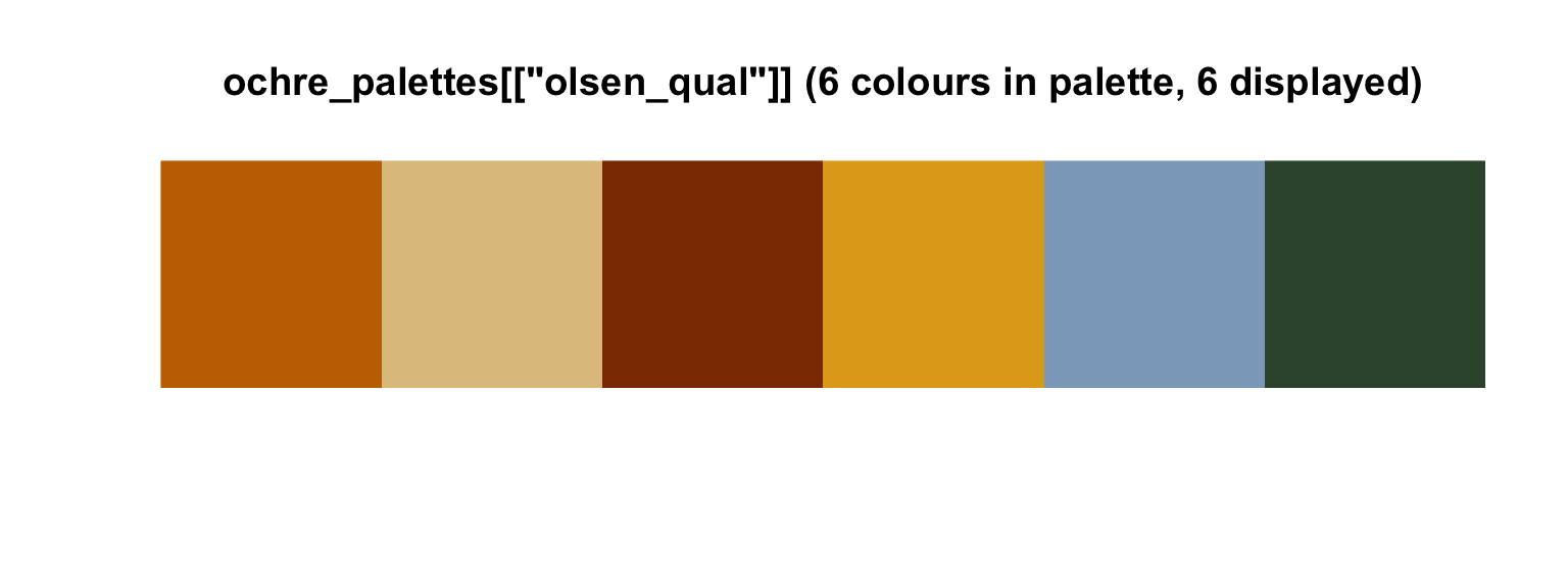
viz_palette(ochre_palettes[["olsen_seq"]])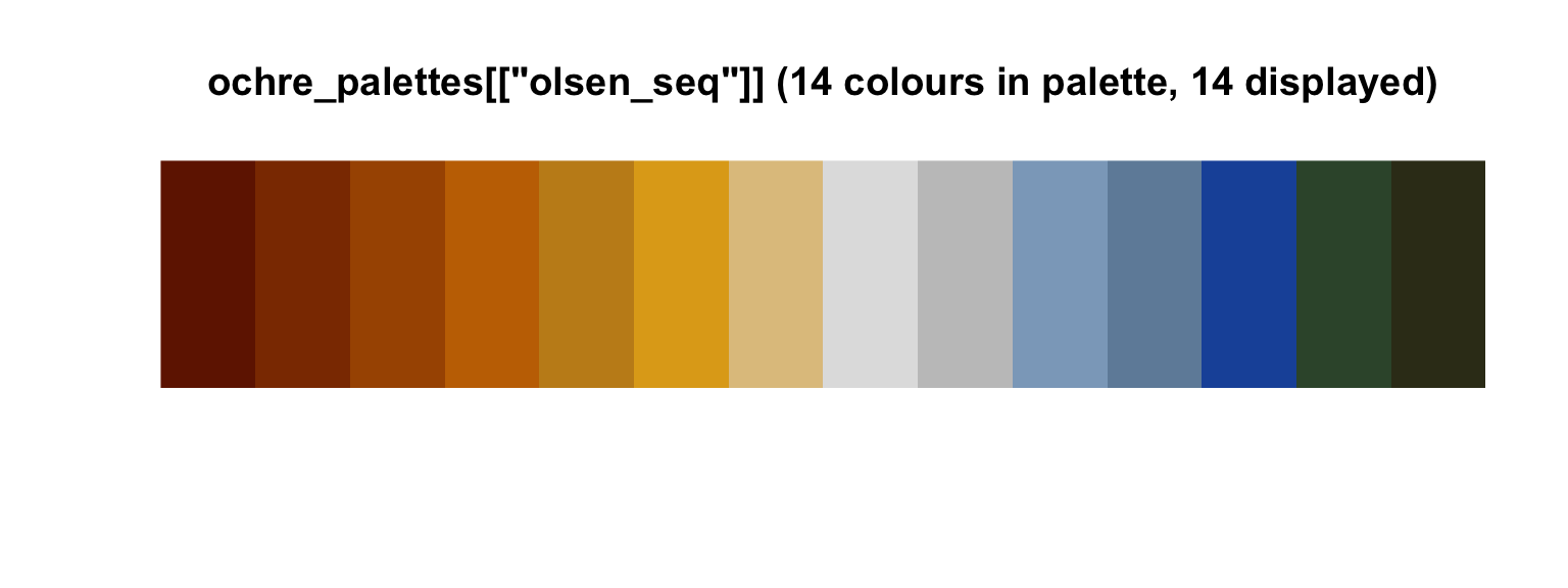
Behold our Figure 8.3.
# these will come in handy with `geom_text()`, below
green_slope <- (fixef(model1)["skeptic", 1] + fixef(model1)[4, 1]) %>% round(digits = 3)
blue_slope  <- fixef(model1)["skeptic", 1] %>% round(digits = 3)

(
  nd <-
  tibble(frame = rep(0:1, times = 2),
         skeptic = rep(c(0, 7), each = 2))
  )
## # A tibble: 4 x 2
## frame skeptic
## <int> <dbl>
## 1 0 0
## 2 1 0
## 3 0 7
## 4 1 7fitted(model1, newdata = nd,
summary = F) %>%
as_tibble() %>%
gather() %>%
mutate(iter = rep(1:4000, times = 4),
frame = rep(rep(0:1, each = 4000),
times = 2),
skeptic = rep(c(0, 7), each = 4000*2)) %>%
ggplot(aes(x = skeptic, y = value,
group = interaction(frame, iter),
color = frame %>% as.character())) +
geom_line(aes(color = frame %>% as.character()),
size = 1/6, alpha = 1/25) +
geom_text(data = tibble(skeptic = c(4, 4.6),
value = c(3.5, 2.6),
frame = 1:0,
iter = 0,
label = c(paste("the slope when frame = 1 is about", green_slope),
paste("the slope when frame = 0 is about", blue_slope)),
angle = c(28, 6)),
aes(label = label, angle = angle)) +
scale_color_manual(NULL, values = ochre_palettes[["olsen_qual"]][(5:6)]) +
scale_x_continuous(breaks = 1:6) +
coord_cartesian(xlim = 1:6,
ylim = 2:4) +
labs(title = "The moderation effect in a spaghetti plot",
subtitle = "Using brms defaults, we have 4000 posterior draws. Much like we have\n4000 draws for each model parameter, when we combine those draws\nacross parameters, we end up with 4000 model equations. The\nconsequence is we can also express the line plot as 4000\nsemitransparent lines, one for each level of our moderator, frame.",
x = expression(paste("Climate Change Skepticism (", italic("X"), ")")),
y = "Strength of Justification for Withholding Aid") +
theme_08 +
theme(legend.position = "none")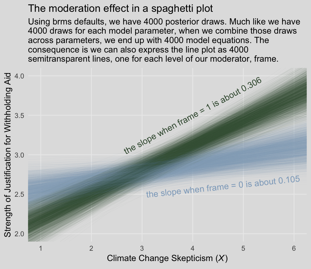
In addition to our fancy Australia-inspired colors, we’ll also play around a bit with spaghetti plots in this chapter. To my knowledge, this use of spaghetti plots is uniquely Bayesian. If you’re trying to wrap your head around what on earth we just did, take a look at the first few rows from posterior_samples() object, post.
post <- posterior_samples(model1)

head(post)
## b_Intercept b_skeptic b_frame b_skeptic:frame sigma lp__
## 1 2.433604 0.10925232 -0.78012292 0.2741745 0.7915912 -261.9281
## 2 2.395932 0.10581691 -0.31127291 0.1787660 0.8438781 -261.6192
## 3 2.424501 0.11975748 -0.54167062 0.1779073 0.7571458 -260.9795
## 4 2.406765 0.09432444 -0.50329667 0.2094752 0.7874562 -260.5686
## 5 2.105076 0.19317602 -0.23817452 0.1183026 0.8268476 -262.7449
## 6 2.201878 0.14910845 0.02174834 0.1016261 0.8216859 -263.8987head() returned six rows, each one corresponding to the credible parameter values from a given posterior draw. The lp__ is uniquely Bayesian and beyond the scope of this project. You might think of sigma as the Bayesian analogue to what the OLS folks often refer to as error or the residual variance. Hayes doesn’t tend to emphasize it in this text, but it’s something you’ll want to pay increasing attention to as you move along in your Bayesian career. All the columns starting with b_ are the regression parameters, the model coefficients or the fixed effects. But anyways, notice that those b_ columns correspond to the four parameter values in formula 8.2 on page 270. Here they are, but reformatted to more closely mimic the text:
- \(\hat{Y}\) = 2.434 + 0.109\(X\) + -0.78\(W\) + 0.274XW
- \(\hat{Y}\) = 2.396 + 0.106\(X\) + -0.311\(W\) + 0.179XW
- \(\hat{Y}\) = 2.425 + 0.12\(X\) + -0.542\(W\) + 0.178XW
- \(\hat{Y}\) = 2.407 + 0.094\(X\) + -0.503\(W\) + 0.209XW
- \(\hat{Y}\) = 2.105 + 0.193\(X\) + -0.238\(W\) + 0.118XW
- \(\hat{Y}\) = 2.202 + 0.149\(X\) + 0.022\(W\) + 0.102XW
Each row of post, each iteration or posterior draw, yields a full model equation that is a credible description of the data—or at least as credible as we can get within the limits of the model we have specified, our priors (which we typically cop out on and just use defaults in this project), and how well those fit when applied to the data at hand. So when we use brms convenience functions like fitted(), we pass specific predictor values through those 4000 unique model equations, which returns 4000 similar but distinct expected \(Y\)-values. So although a nice way to summarize those 4000 values is with summaries such as the posterior mean/median and 95% intervals, another way is to just plot an individual regression line for each of the iterations. That is what’s going on when we depict out models with a spaghetti plot.
The thing I like about spaghetti plots is that they give a three-dimensional sense of the posterior. Note that each individual line is very skinny and semitransparent. When you pile a whole bunch of them atop each other, the peaked or most credible regions of the posterior are the most saturated in color. Less credible posterior regions almost seamlessly merge into the background. Also, note how the combination of many similar but distinct straight lines results in a bowtie shape. Hopefully this clarifies where that shape’s been coming from when we use geom_ribbon() to plot the 95% intervals.
But anyways, you could recode frame in a number of ways, including ifelse() or, in this case, by simple arithmetic.
disaster <-
  disaster %>%
  mutate(frame_ep = 1 - frame)
With frame_ep in hand, we’re ready to refit the model.
model2 <-
  update(model1, newdata = disaster,
         formula = justify ~ 1 + skeptic + frame_ep + frame_ep:skeptic,
chains = 4, cores = 4)print(model2)## Family: gaussian
## Links: mu = identity; sigma = identity
## Formula: justify ~ skeptic + frame_ep + skeptic:frame_ep
## Data: disaster (Number of observations: 211)
## Samples: 4 chains, each with iter = 2000; warmup = 1000; thin = 1;
## total post-warmup samples = 4000
##
## Population-Level Effects:
## Estimate Est.Error l-95% CI u-95% CI Eff.Sample Rhat
## Intercept 1.89 0.16 1.56 2.20 2201 1.00
## skeptic 0.31 0.04 0.23 0.39 2197 1.00
## frame_ep 0.56 0.23 0.13 1.01 1779 1.00
## skeptic:frame_ep -0.20 0.06 -0.31 -0.09 1731 1.00
##
## Family Specific Parameters:
## Estimate Est.Error l-95% CI u-95% CI Eff.Sample Rhat
## sigma 0.82 0.04 0.75 0.90 2919 1.00
##
## Samples were drawn using sampling(NUTS). For each parameter, Eff.Sample
## is a crude measure of effective sample size, and Rhat is the potential
## scale reduction factor on split chains (at convergence, Rhat = 1).Our results match nicely with the formula on page 275.
If you want to follow along with Hayes on pate 276 and isolate the 95% credible intervals for the skeptic parameter, you can use posterior_interval().
posterior_interval(model2)["b_skeptic", ] %>% round(digits = 3)## 2.5% 97.5%
## 0.227 0.388