2.7 Multicategorical antecedent variables
partyid is coded 1 = Democrat 2 = Independent 3 = Repuclican. You can get a count of the cases within a give partyid like this:
glbwarm %>%
  group_by(partyid) %>%
  count()
#> # A tibble: 3 x 2
#> # Groups:   partyid [3]
#>   partyid     n
#>     <int> <int>
#> 1       1   359
#> 2       2   192
#> 3       3   264
We can get grouped means for govact like this:
glbwarm %>%
  group_by(partyid) %>%
  summarize(mean_support_for_governmental_action = mean(govact))
#> # A tibble: 3 x 2
#>   partyid mean_support_for_governmental_action
#>     <int>                                <dbl>
#> 1       1                                 5.06
#> 2       2                                 4.61
#> 3       3                                 3.92
We can make dummies with the ifelse() function. We’ll just go ahead and do that right within the brm() function.
model6 <-
  brm(data = glbwarm %>%
        mutate(Democrat = ifelse(partyid == 1, 1, 0),
               Republican = ifelse(partyid == 3, 1, 0)),
      family = gaussian,
      govact ~ 1 + Democrat + Republican,
chains = 4, cores = 4)fixef(model6)
#> Estimate Est.Error Q2.5 Q97.5
#> Intercept 4.607 0.0929 4.426 4.786
#> Democrat 0.458 0.1140 0.232 0.683
#> Republican -0.684 0.1224 -0.913 -0.436The intercept is the stand-in for Independents and the other two coefficients are difference scores.
The \(R^2\) is okay:
bayes_R2(model6) %>% round(digits = 3)
#>    Estimate Est.Error  Q2.5 Q97.5
#> R2    0.133     0.021 0.093 0.175
There’s no need to compute an \(F\)-test on our \(R^2\). The posterior mean and it’s 95% intervals are well away from zero. But you could use your bayes_R2(model6, summary = F) plotting skills from above to more fully inspect the posterior if you’d like.
We could also use information criteria. One method would be to compare the WAIC or LOO value of model6 with an intercept-only model. First, we’ll need to fit that model.
model7 <-
  update(model6,
         govact ~ 1,
         chains = 4, cores = 4)
If we just put both models into waic(), we can side step the need to save their outputs as objects which we then put into compare_ic().
waic(model6, model7)
#>                 WAIC   SE
#> model6          2707 40.1
#> model7          2818 42.7
#> model6 - model7 -110 20.8
The WAIC comparison suggests model6, the one with the partyid dummies, is an improvement over the simple intercept-only model. Another way to compare the information criteria is with AIC-type weighting. The brms package offers a variety of weighting methods via the model_weights() function.
MWs <- model_weights(model6, model7, weights = "waic")

MWs
#>   model6   model7
#> 1.00e+00 1.14e-24
If you’re not a fan of scientific notation, you can put the results in a tibble and look at them on a plot.
MWs %>%
  as.data.frame() %>%
  rownames_to_column() %>%

  ggplot(aes(x = ., y = rowname)) +
  geom_point() +
  labs(subtitle = "The weights should sum to 1. In this case virtually all the weight is placed\nin model6. Recall, that these are RELATIVE weights. Add another\nmodel fit into the mix and the weights might well change.",
       x = "WAIC weight", y = NULL) +
  theme_bw() +
  theme(axis.ticks.y = element_blank())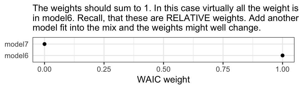
You could, of course, do all this with the LOO.