13.2 Looking at the components of the indirect effect of \(X\)
13.2.1 Examining the first stage of the mediation process.
When making a newdata object to feed into fitted() with more complicated models, it can be useful to review the model formula like so:
model1$formula## respappr ~ 1 + D1 + D2 + sexism + D1:sexism + D2:sexism
## liking ~ 1 + D1 + D2 + respappr + sexism + D1:sexism + D2:sexismNow we’ll prep for and make our version of Figure 13.3.
nd <-
  tibble(D1 = rep(c(1/3, -2/3, 1/3), each = 30),
         D2 = rep(c(1/2, 0, -1/2), each = 30),
         sexism = rep(seq(from = 3.5, to = 6.5, length.out = 30),
                      times = 3))

model1_fitted <-
  fitted(model1,
       newdata = nd,
       resp = "respappr") %>%
  as_tibble() %>%
  bind_cols(nd) %>%
  mutate(condition = ifelse(D2 == 0, "No Protest",
                            ifelse(D2 == -1/2, "Individual Protest", "Collective Protest"))) %>%
  mutate(condition = factor(condition, levels = c("No Protest", "Individual Protest", "Collective Protest")))

protest <-
  protest %>%
  mutate(condition = ifelse(protest == 0, "No Protest",
                            ifelse(protest == 1, "Individual Protest", "Collective Protest"))) %>%
  mutate(condition = factor(condition, levels = c("No Protest", "Individual Protest", "Collective Protest")))

model1_fitted %>%
  ggplot(aes(x = sexism, group = condition)) +
  geom_ribbon(aes(ymin = Q2.5, ymax = Q97.5),
              linetype = 3, color = "white", fill = "transparent") +
  geom_line(aes(y = Estimate), color = "white") +
  geom_point(data = protest, aes(x = sexism, y = respappr),
             color = "red", size = 2/3) +
  coord_cartesian(xlim = 4:6) +
  labs(x = expression(paste("Perceived Pervasiveness of Sex Discrimination in Society (", italic(W), ")")),
       y = expression(paste("Perceived Appropriateness of Response (", italic(M), ")"))) +
  theme_black() +
  theme(panel.grid = element_blank()) +
  facet_wrap(~condition)
In order to get the \(\Delta R^2\) distribution analogous to the change in \(R^2\) \(F\)-test Hayes discussed on page 482, we’ll have to first refit the model without the interaction for the \(M\) criterion. Here are the sub-models.
m_model <- bf(respappr ~ 1 + D1 + D2 + sexism)
y_model <- bf(liking   ~ 1 + D1 + D2 + respappr + sexism + D1:sexism + D2:sexism)
Now we fit model2.
model2 <-
  brm(data = protest, family = gaussian,
      m_model + y_model + set_rescor(FALSE),
      chains = 4, cores = 4)
With model2 in hand, we’re ready to compare \(R^2\) distributions.
R2s <-
  bayes_R2(model1, resp = "respappr", summary = F) %>%
  as_tibble() %>%
  rename(model1 = R2_respappr) %>%
  bind_cols(
    bayes_R2(model2, resp = "respappr", summary = F) %>%
      as_tibble() %>%
      rename(model2 = R2_respappr)
  ) %>%
  mutate(difference = model1 - model2)

R2s %>%
  ggplot(aes(x = difference)) +
  geom_halfeyeh(aes(y = 0), fill = "grey50", color = "white",
                point_interval = median_qi, .prob = 0.95) +
  scale_x_continuous(breaks = median_qi(R2s$difference, .prob = .95)[1, 1:3],
                     labels = median_qi(R2s$difference, .prob = .95)[1, 1:3] %>% round(2)) +
  scale_y_continuous(NULL, breaks = NULL) +
  xlab(expression(paste(Delta, italic(R)^2))) +
  theme_black() +
  theme(panel.grid = element_blank())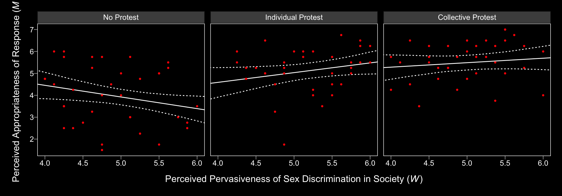
And we might also compare the models by their information criteria.
loo(model1, model2)## LOOIC SE
## model1 760.10 29.56
## model2 765.47 29.71
## model1 - model2 -5.37 7.96waic(model1, model2)## WAIC SE
## model1 759.74 29.47
## model2 765.32 29.71
## model1 - model2 -5.58 7.96The Bayesian \(R^2\), the LOO-CV, and the WAIC all suggest there’s little difference between the two models with respect to their predictive utility. In such a case, I’d lean on theory to choose between them. If inclined, one could also do Bayesian model averaging.
Within our Bayesian modeling paradigm, we don’t have a direct analogue to the \(F\)-tests Hayes presented on page 483. But a little fitted() and follow-up wrangling will give us some difference scores.
# we need new `nd` data
nd <-
  tibble(D1 = rep(c(1/3, -2/3, 1/3), each = 3),
         D2 = rep(c(1/2, 0, -1/2), each = 3),
         sexism = rep(c(4.250, 5.120, 5.896), times = 3))

# this time we'll use `summary = F`
model1_fitted <-
  fitted(model1,
       newdata = nd,
       resp = "respappr",
       summary = F) %>%
  as_tibble() %>%
  gather() %>%
  mutate(condition = rep(c("Collective Protest", "No Protest", "Individual Protest"),
                         each = 3*4000),
         sexism = rep(c(4.250, 5.120, 5.896), times = 3) %>% rep(., each = 4000),
         iter = rep(1:4000, times = 9)) %>%
  select(-key) %>%
  spread(key = condition, value = value) %>%
  mutate(`Individual Protest - No Protest` = `Individual Protest` - `No Protest`,
         `Collective Protest - No Protest` = `Collective Protest` - `No Protest`,
         `Collective Protest - Individual Protest` = `Collective Protest` - `Individual Protest`)

# a tiny bit more wrangling and we're ready to plot the difference distributions
model1_fitted %>%
  select(sexism, contains("-")) %>%
  gather(key, value, -sexism) %>%

  ggplot(aes(x = value)) +
  geom_halfeyeh(aes(y = 0), fill = "grey50", color = "white",
                point_interval = median_qi, .prob = 0.95) +
  geom_vline(xintercept = 0, color = "grey25", linetype = 2) +
  scale_y_continuous(NULL, breaks = NULL) +
  facet_grid(sexism~key) +
  theme_black() +
  theme(panel.grid = element_blank())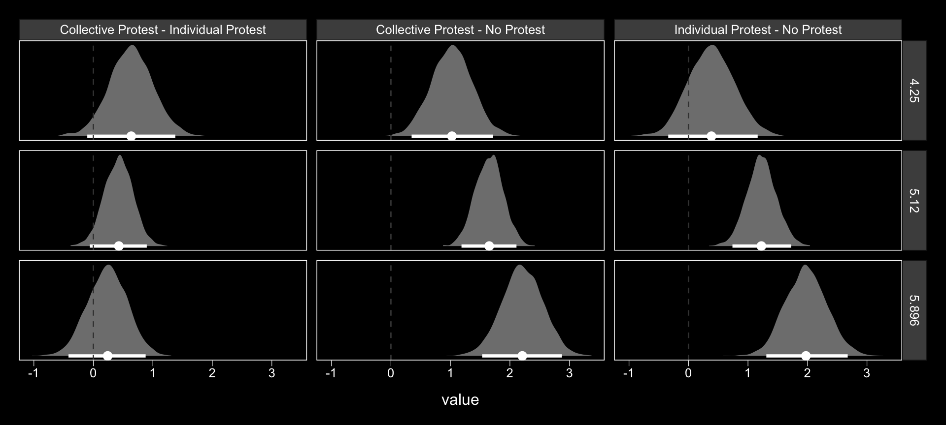
Now we have model1_fitted, it’s easy to get the typical numeric summaries for the differences.
model1_fitted %>%
  select(sexism, contains("-")) %>%
  gather(key, value, -sexism) %>%
  group_by(key, sexism) %>%
  summarize(mean = mean(value),
            ll = quantile(value, probs = .025),
            ul = quantile(value, probs = .975)) %>%
  mutate_if(is.double, round, digits = 3)
## # A tibble: 9 x 5
## # Groups: key [3]
## key sexism mean ll ul
## <chr> <dbl> <dbl> <dbl> <dbl>
## 1 Collective Protest - Individual Protest 4.25 0.636 -0.102 1.38
## 2 Collective Protest - Individual Protest 5.12 0.424 -0.059 0.898
## 3 Collective Protest - Individual Protest 5.90 0.234 -0.418 0.879
## 4 Collective Protest - No Protest 4.25 1.02 0.348 1.72
## 5 Collective Protest - No Protest 5.12 1.65 1.19 2.11
## 6 Collective Protest - No Protest 5.90 2.21 1.53 2.87
## 7 Individual Protest - No Protest 4.25 0.388 -0.34 1.16
## 8 Individual Protest - No Protest 5.12 1.23 0.739 1.73
## 9 Individual Protest - No Protest 5.90 1.98 1.31 2.68The three levels of Collective Protest - Individual Protest correspond nicely with some of the analyses Hayes presented on pages 484–486. However, they don’t get at the differences Hayes expressed as \(\theta_{D_{1}\rightarrow M}\) to . For those, we’ll have to work directly with the posterior_samples().
post <- posterior_samples(model1)

post %>%
  mutate(`Difference in how Catherine's behavior is perceived between being told she protested or not when W is 4.250` = b_respappr_D1 + `b_respappr_D1:sexism`*4.250,
         `Difference in how Catherine's behavior is perceived between being told she protested or not when W is 5.210` = b_respappr_D1 + `b_respappr_D1:sexism`*5.120,
         `Difference in how Catherine's behavior is perceived between being told she protested or not when W is 5.896` = b_respappr_D1 + `b_respappr_D1:sexism`*5.896) %>%
  select(contains("Difference")) %>%
  gather() %>%
  group_by(key) %>%
  summarize(mean = mean(value),
            ll = quantile(value, probs = .025),
            ul = quantile(value, probs = .975)) %>%
  mutate_if(is.double, round, digits = 3)
## # A tibble: 3 x 4
## key mean ll ul
## <chr> <dbl> <dbl> <dbl>
## 1 Difference in how Catherine's behavior is perceived between being told she pro… 0.706 0.086 1.34
## 2 Difference in how Catherine's behavior is perceived between being told she pro… 1.44 1.02 1.85
## 3 Difference in how Catherine's behavior is perceived between being told she pro… 2.09 1.51 2.6913.2.2 Estimating the second stage of the mediation process.
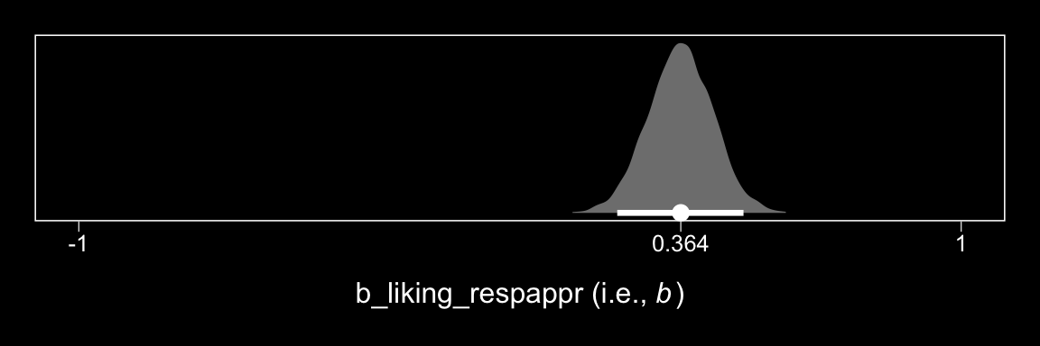
Here’s \(b\).
post %>%

  ggplot(aes(x = b_liking_respappr)) +
  geom_halfeyeh(aes(y = 0), fill = "grey50", color = "white",
                point_interval = median_qi, .prob = 0.95) +
  scale_x_continuous(breaks = c(-1, median(post$b_liking_respappr), 1),
                     labels = c(-1,
                                median(post$b_liking_respappr) %>% round(3),
                                1)) +
  scale_y_continuous(NULL, breaks = NULL) +
  coord_cartesian(xlim = -1:1) +
  xlab(expression(paste("b_liking_respappr (i.e., ", italic(b), ")"))) +
  theme_black() +
  theme(panel.grid = element_blank())