8.4 Weighted linear regression
8.4.1 Fitting the model
To carry out a linear regression that incorporates a survey design, use svyglm() with family=gaussian(). “Gaussian” means “normally distributed” so this is specifying a model with an outcome that, given the predictors, is normally distributed, which is equivalent to specifying a linear regression with normally distributed errors. See, for example, Lumley and Scott (2017) and for further reading about fitting regression models to complex survey data.
After fitting the model, use summary(), confint(), and car::Anova(, type = 3, test.statistic = "F") to view the regression coefficients, their 95% confidence intervals, and p-values. Each of these functions has an option to change the DF to the design DF. Finally, table the regression results using tbl_regression(). There is an option to change the DF in tbl_regression(), but it only applies to the overall p-values for categorical predictors, so the confidence intervals and remaining p-values in the table are based on default DF rather than the design DF. See the “Details” section in ?summary.svyglm for information regarding the default DF.
Example 8.1 (continued): Regress the outcome fasting glucose (LBDGLUSI) on the predictors waist circumference (BMXWAIST), smoking status (smoker), age (RIDAGEYR), gender (RIAGENDR), race/ethnicity (RIDRETH3), and income (income), correctly incorporating the NHANES survey design to obtain estimates representative of the population. Use the NHANES 2017-2018 fasting subset survey design we have been working with in this chapter (design.FST.nomiss).
fit.ex8.1 <- svyglm(LBDGLUSI ~ BMXWAIST + smoker + RIDAGEYR +
                      RIAGENDR + race_eth + income,
                 family=gaussian(), design=design.FST.nomiss)
When calling summary(), confint(), and car::Anova() to summarize the results, use the df.resid, ddf, and error.df options, respectively, to specify the design DF for confidence intervals and hypothesis tests. To ensure you are using the same design as was used in the regression, extract the design from the svyglm object as fit$survey.design.
round(
  cbind(
    summary(fit.ex8.1, df.resid = degf(fit.ex8.1$survey.design))$coef,
    confint(fit.ex8.1, ddf      = degf(fit.ex8.1$survey.design))
  )
, 4)
## Estimate Std. Error t value Pr(>|t|) 2.5 % 97.5 %
## (Intercept) 3.3890 0.3542 9.5670 0.0000 2.6340 4.1441
## BMXWAIST 0.0221 0.0031 7.0544 0.0000 0.0154 0.0288
## smokerPast 0.1914 0.0961 1.9916 0.0649 -0.0134 0.3963
## smokerCurrent 0.0055 0.1103 0.0499 0.9609 -0.2297 0.2407
## RIDAGEYR 0.0210 0.0020 10.2867 0.0000 0.0166 0.0253
## RIAGENDRFemale -0.3331 0.0684 -4.8694 0.0002 -0.4789 -0.1873
## race_ethNon-Hispanic White -0.3448 0.1461 -2.3599 0.0322 -0.6561 -0.0334
## race_ethNon-Hispanic Black -0.2577 0.1565 -1.6470 0.1203 -0.5912 0.0758
## race_ethNon-Hispanic Other -0.1095 0.1381 -0.7928 0.4402 -0.4040 0.1849
## income$25,000 to <$55,000 -0.1437 0.1414 -1.0162 0.3256 -0.4452 0.1577
## income$55,000+ -0.1224 0.0895 -1.3674 0.1917 -0.3132 0.0684## Analysis of Deviance Table (Type III tests)
##
## Response: LBDGLUSI
## Df F Pr(>F)
## (Intercept) 1 91.53 0.000000089 ***
## BMXWAIST 1 49.77 0.000003909 ***
## smoker 2 2.09 0.1584
## RIDAGEYR 1 105.82 0.000000034 ***
## RIAGENDR 1 23.71 0.0002 ***
## race_eth 3 3.00 0.0636 .
## income 2 1.03 0.3793
## Residuals 15
## ---
## Signif. codes: 0 '***' 0.001 '**' 0.01 '*' 0.05 '.' 0.1 ' ' 1To table these results, use the tbl_regression() function in gtsummary after adding test.statistic = "F" in add_global_p(). The results are shown in Table 8.3.
Warning: There is no option in tbl_regression() to change the DF to make the confidence intervals and p-values for the individual regression coefficients be based on the design DF. There is an option in add_global_p() to change the DF for the Type III tests (commented out in the code below); however, using that option will lead to p-values that do not match between the overall (Type III) test for a binary predictor and the test for the single term in the model for that binary predictor. The code below uses R’s default DF throughout. If, instead, you want to use the design DF throughout, uncomment the error.df row below and export the table (see Sections 3.3.2 and 3.3.3). Then, in a word processing program, edit the confidence intervals and p-values for each regression coefficient, replacing them with those you computed above using the design DF.
library(gtsummary)
TABLE <- fit.ex8.1 %>%
  tbl_regression(intercept = T,
                 estimate_fun = function(x) style_sigfig(x, digits = 3),
                 pvalue_fun   = function(x) style_pvalue(x, digits = 3),
                 label  = list(BMXWAIST ~ "Waist Circumference (cm)",
                               smoker   ~ "Smoking Status",
                               RIDAGEYR ~ "Age (years)",
                               RIAGENDR ~ "Gender",
                               race_eth ~ "Race/Ethnicity",
                               income   ~ "Annual Income")) %>%
  add_global_p(keep = T, test.statistic = "F"
  # Uncomment to use design df for Type III test p-values
  # (but then they will not match the regression term p-values for
  #  binary predictors)
  #             , error.df = degf(fit.ex8.1$survey.design)
                                 ) %>%
  modify_caption(
"Weighted linear regression results for fasting glucose (mmol/L)")| Characteristic | Beta | 95% CI | p-value |
|---|---|---|---|
| (Intercept) | 3.39 | 2.48, 4.30 | <0.001 |
| Waist Circumference (cm) | 0.022 | 0.014, 0.030 | <0.001 |
| Smoking Status | 0.219 | ||
| Never | — | — | |
| Past | 0.191 | -0.056, 0.438 | 0.103 |
| Current | 0.006 | -0.278, 0.289 | 0.962 |
| Age (years) | 0.021 | 0.016, 0.026 | <0.001 |
| Gender | 0.005 | ||
| Male | — | — | |
| Female | -0.333 | -0.509, -0.157 | 0.005 |
| Race/Ethnicity | 0.134 | ||
| Hispanic | — | — | |
| Non-Hispanic White | -0.345 | -0.720, 0.031 | 0.065 |
| Non-Hispanic Black | -0.258 | -0.660, 0.145 | 0.160 |
| Non-Hispanic Other | -0.110 | -0.465, 0.246 | 0.464 |
| Annual Income | 0.421 | ||
| <$25,000 | — | — | |
| $25,000 to <$55,000 | -0.144 | -0.507, 0.220 | 0.356 |
| $55,000+ | -0.122 | -0.353, 0.108 | 0.230 |
| Abbreviation: CI = Confidence Interval | |||
Conclusion: After adjusting for age, gender, race/ethnicity, income, and each other, waist circumference is significantly associated with fasting glucose (B = 0.022; 95% CI = 0.014, 0.030; p <.001) but smoking status is not (p = .219).
8.4.2 Prediction
As was the case with glm(), predict() applied to a svyglm() object does not return a CI. Instead, use svycontrast_design_df() (in Functions_rmph.R, which you loaded at the beginning of this chapter), a modified version of svycontrast() with a DF option, which is similar to gmodels::estimable(). See Chapter 6.8 for how to specify the second argument to get the estimate of interest.
Example 8.1 (continued): What is the estimated population mean fasting glucose among individuals with a waist circumference of 120 cm, who have never smoked, are age 35 years, female, and Hispanic, and have an annual income from $25,000 to <$55,000?
# Always include the intercept for estimation
# Specify a 1 for the intercept, a # for each continuous predictor
# and a 1 for each non-reference level of a categorical variable.
# If a predictor is at its reference level, it should be left out.
svycontrast_design_df(fit.ex8.1,
                      c("(Intercept)"               = 1,
                        "BMXWAIST"                  = 120,
                        "RIDAGEYR"                  = 35,
                        "RIAGENDRFemale"            = 1,
                        "income$25,000 to <$55,000" = 1))
## est lower upper
## 1 6.302 6.018 6.585Conclusion: The estimated population mean fasting glucose among such individuals is 6.30 mmol/L (95% CI = 6.02, 6.59).
8.4.3 Interactions
The syntax for including an interaction in svyglm() is exactly as in lm(): add X:Z to include an interaction between X and Z.
Example 8.2: Does the association between the outcome fasting glucose (LBDGLUSI) and waist circumference (BMXWAIST) depend on gender (RIAGENDR), adjusted for smoking status, age, race, and income? Correctly incorporate the NHANES survey design to obtain an estimate of the waist circumference slope for each gender that is generalizable to the population.
fit.ex8.2 <- svyglm(LBDGLUSI ~ BMXWAIST + smoker + RIDAGEYR +
                      RIAGENDR + race_eth + income + BMXWAIST:RIAGENDR,
                 family=gaussian(), design=design.FST.nomiss)

round(
  cbind(
    summary(fit.ex8.2,
              df.resid=degf(fit.ex8.2$survey.design))$coef,
    confint(fit.ex8.2,
              ddf=degf(fit.ex8.2$survey.design))
  )
, 4)
## Estimate Std. Error t value Pr(>|t|) 2.5 % 97.5 %
## (Intercept) 3.2130 0.4739 6.7793 0.0000 2.2028 4.2231
## BMXWAIST 0.0239 0.0048 4.9532 0.0002 0.0136 0.0342
## smokerPast 0.1937 0.0991 1.9546 0.0695 -0.0175 0.4050
## smokerCurrent 0.0102 0.1151 0.0886 0.9305 -0.2351 0.2555
## RIDAGEYR 0.0208 0.0023 9.2184 0.0000 0.0160 0.0256
## RIAGENDRFemale -0.0256 0.5868 -0.0437 0.9657 -1.2765 1.2252
## race_ethNon-Hispanic White -0.3429 0.1447 -2.3705 0.0316 -0.6513 -0.0346
## race_ethNon-Hispanic Black -0.2495 0.1573 -1.5866 0.1335 -0.5848 0.0857
## race_ethNon-Hispanic Other -0.1085 0.1374 -0.7898 0.4420 -0.4014 0.1843
## income$25,000 to <$55,000 -0.1447 0.1409 -1.0269 0.3207 -0.4450 0.1556
## income$55,000+ -0.1257 0.0911 -1.3795 0.1880 -0.3198 0.0685
## BMXWAIST:RIAGENDRFemale -0.0031 0.0055 -0.5592 0.5843 -0.0147 0.0086The p-value for BMXWAIST:RIAGENDRFemale is >0.05, so the interaction is not statistically significant.
To estimate the waist circumference slope at each level of gender, use svycontrast_design_df() (in Functions_rmph.R, which you loaded at the beginning of this chapter). See Section 5.10.7 for how to specify the second argument to get the estimates of interest.
# Estimate slope at each level of other variable, along with a CI
# using the design DF (the default)
rbind(
  "BMXWAIST @ Male"   = svycontrast_design_df(fit.ex8.2,
                              c("BMXWAIST"                = 1)),
  "BMXWAIST @ Female" = svycontrast_design_df(fit.ex8.2,
                              c("BMXWAIST"                = 1,
                                "BMXWAIST:RIAGENDRFemale" = 1))
)
## est lower upper
## BMXWAIST @ Male 0.02393 0.01363 0.03423
## BMXWAIST @ Female 0.02088 0.01336 0.02840Conclusion: After incorporating the NHANES complex survey design, the association between waist circumference and fasting glucose was not significantly different between males and females (p = .584; slope for males = 0.024; slope for females = 0.021).
8.4.4 Visualize the weighted unadjusted relationships
Use svyplot() to visualize the weighted unadjusted relationships between predictors and the outcome using bubble plots, with points representing more individuals in the population plotted with larger circles. This function works for both continuous and categorical predictors (Figures 8.4 and 8.5, respectively). For a continuous predictor, use svysmooth() to superimpose an estimate of the mean outcome vs. the predictor that does not assume linearity.
# Plot for continuous predictor
svyplot(LBDGLUSI ~ BMXWAIST, design.FST.nomiss,
        ylab = "Fasting Glucose (mmol/L)",
        xlab = "Waist Circumference (cm)")
# Fit unadjusted model
fit.wc <- svyglm(LBDGLUSI ~ BMXWAIST,
                 family=gaussian(), design=design.FST.nomiss)
# Add line
abline(fit.wc, col = "red", lwd = 2)
# Add smoother
lines(svysmooth(fit.wc$formula,
                fit.wc$survey.design,
                df = 5),
      col = "blue", lwd = 2, lty = 2)
legend("topright", c("Regression line", "Smoother"),
       title = "Weighted estimate",
       col = c("red", "blue"), lwd = c(2,2), lty = c(1,2),
       bty = "n", seg.len = 5)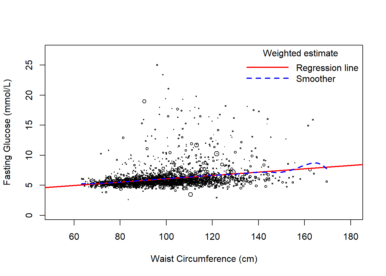
Figure 8.4: Weighted scatterplot of outcome vs. a continuous predictor
# Plot for categorical predictor
svyplot(LBDGLUSI ~ smoker, design.FST.nomiss,
        ylab = "Fasting Glucose (mmol/L)",
        xlab = "Smoking Status",
        xaxt = "n")
axis(1, at = 1:3, labels = levels(nhanes.mod$smoker))
# Fit unadjusted model
fit.smoker <- svyglm(LBDGLUSI ~ smoker,
                 family=gaussian(), design=design.FST.nomiss)
# Compute means
MEANS <- as.numeric(
  predict(fit.smoker,
          data.frame(smoker=levels(nhanes.mod$smoker)))
)
# Add points and lines
points(1:length(MEANS), MEANS, col = "red", pch = 20, cex = 2)
lines( 1:length(MEANS), MEANS, col = "red")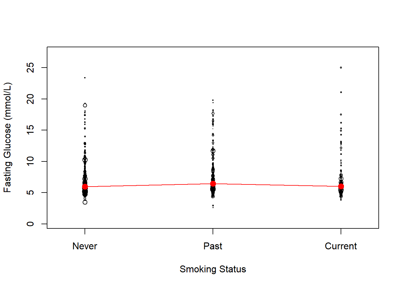
Figure 8.5: Weighted plot of outcome vs. a categorical predictor