6.3 Why not use linear regression for a binary outcome?

Example 6.1 (continued): Figure 6.1 displays the linear regression fit for simulated data from 60 individuals aged 20 to 80 years where \(Y\) = coronary heart disease (CHD) status and \(X\) = age. The possible values for \(Y\) are “yes” and “no” coded as \(Y = 1\) and \(0\), respectively. The gray dots at \(Y = 1\) (along the top of the figure) are plotted at the ages of individuals with CHD, while the dots at \(Y = 0\) (along the bottom of the figure) are for those without CHD. The solid line is the linear regression line, which attempts to estimate the proportion of CHD = Yes (the mean outcome) as a function of age using a straight line. The dashed line is a smoother which tracks the observed proportion without any constraint on its shape.

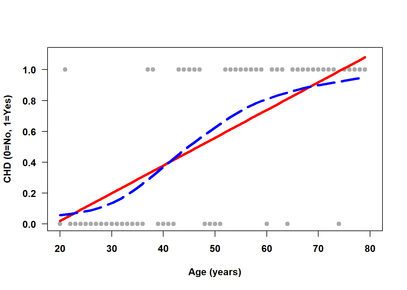
Figure 6.1: Linear regression does not fit well for a binary outcome

A straight line is not a good fit to this data in the sense that most of the points are very far from the line. However, it turns out to be not a terrible fit when comparing it to the relationship between the proportion of CHD = Yes and age (the dashed line). However, in general, logistic regression does even better at estimating the proportion.

Logistic regression models the mean (the probability of \(Y = 1\)) using the complicated looking logit function \(\ln{(p/(1-p))}\) on the left-hand side of the equation. Why not have \(Y\) or \(p\) on the left-hand side? One reason is that, ideally, the range of possible values on the left-hand side should match that of the right-hand side. The right-hand side of the model equation is \(\beta_0 + \beta_1 X_1 + \beta_2 X_2 + \ldots + \beta_K X_K\) and can take on any value from \(-\infty\) to \(\infty\), whereas \(Y\) can only be 0 or 1 and \(p\) must be in the range 0 to 1. However, the logit of \(p\), \(\ln{(p/(1-p))}\), can take on any value, and so matches the right-hand side.

When transformed back to the probability scale, logistic regression fits an S-shaped curve that estimates the proportion of 1’s at a given value of the predictor. Figure 6.2 demonstrates how the logistic regression fit (solid line) closely tracks the smoother (dashed line) and the predicted probabilities are all in [0, 1]. At the highest observed ages, however, the height of the estimated linear regression line (in Figure 6.1) is greater than 1, resulting in predictions outside of [0, 1].

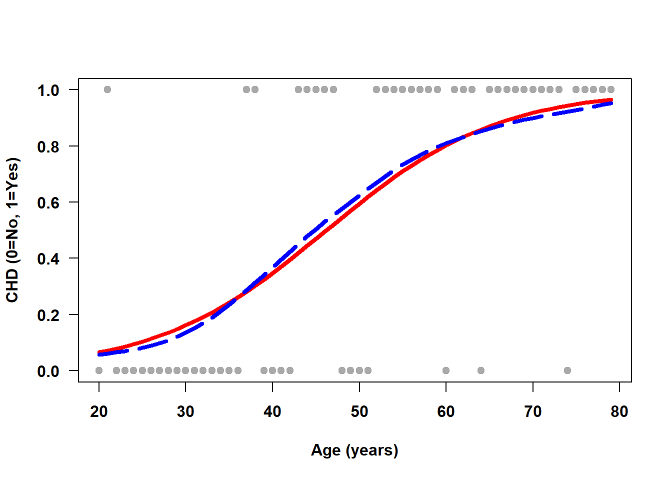
Figure 6.2: Logistic regression fits an S-shaped curve modeling P(Y = 1)