7.16 Proportional hazards assumption
The reason Cox regression is called Cox “proportional hazards” (PH) regression is that the standard form of the model assumes the hazards for any two individuals have the same proportion at all times. Thus, the PH assumption implies the HR measuring the effect of any predictor is constant over time.
Consider two individuals who differ by one unit in \(X_K\) and do not differ in any other predictor in the model. Their Cox model hazard functions are the following:
\[\begin{array}{lcl} h(t \vert X_1 = x_1, ..., X_K = x_K+1) & = & h_0(t) e^{\beta_1 x_1 + \ldots + \beta_K(x_K+1)} \\ h(t \vert X_1 = x_1, ..., X_K = x_K) & = & h_0(t) e^{\beta_1 x_1 + \ldots + \beta_K x_K} \end{array}\]
Taking the ratio of these, everything cancels out except \(e^{\beta_K}\), the AHR for \(X_K\), a quantity which does not depend on time. In fact, you could plug in any two sets of predictor values, differing on any or all of the predictors, and the ratio of the hazards would not depend on time. The hazard \(h(t)\) itself can increase or decrease over time because the baseline hazard \(h_0(t)\) varies with time. However, the ratio of hazards comparing any two individuals is constant because \(h_0(t)\) does not vary between individuals and so cancels out in the ratio.
A violation of the PH assumption does not mean we cannot use Cox regression, just that we need to modify it slightly to account for non-proportional hazards, typically by including an interaction between a predictor and time or by stratifying by a predictor.
7.16.1 Checking the proportional hazards assumption
Suppose we think the HR for \(X_k\) varies linearly with time. This means that instead of having \(\beta_k X_k\) in the model equation, we would have \(\beta_k(t) X_k\) where \(\beta_k(t) = \beta_{k_1} + \beta_{k_2} t\). More generally, \(\beta(t)\) could take on any form. The cox.zph() (Grambsch and Therneau 1994) function checks the PH assumption by comparing the PH model for each predictor to a model that allows that predictor’s regression coefficient to vary smoothly with time, where “smoothly” means the alternative model does not assume a specific form for the time trajectory.
Example 7.6 (continued): Check each predictor for non-proportional hazards in the model we fit for Example 7.6.
To be able to screen each component of a categorical predictor that has \(L > 2\) levels, we must replace the factor version of the variable with the corresponding \(L-1\) indicator variables. Although not necessary at this step, we will also replace each binary categorical variable with an indicator variable as we may need the indicator variable version when we relax the PH assumption in Section 7.16.3.
When you enter a factor variable into a regression model, R automatically creates indicator variables and includes them in the model, leaving out the one for the reference level. The resulting indicator variables can be extracted from a model using the model.matrix() function. Applying this function to our Cox model fit results in a matrix. The following shows the first few rows.
##   RF_PPTERMYes MAGER MRACEHISPNH Black MRACEHISPNH Other MRACEHISPHispanic DMARUnmarried
## 1            0    35                 0                 0                 1             0
## 2            1    28                 0                 0                 0             1
## 3            0    22                 1                 0                 0             1
## 4            0    19                 0                 0                 1             1
## 5            0    30                 0                 0                 0             0
## 6            0    20                 0                 1                 0             1
Extract the indicator variables and assign them to variables inside the dataset and re-fit the model.
NOTES:
- Pay careful attention to how the columns of the model matrix are spelled. In this example, some have spaces (e.g., “MRACEHISPNH Black”). When you create variables in the code below, the strings inside the
[,]s on the right must be spelled exactly as they appear in the model matrix. - This method of extracting indicator variables and adding them to a dataset only works correctly with a complete case dataset. If the dataset used to fit the model was not complete, create a complete-case dataset and re-fit the model before proceeding.
# Extract indicator variables and add to dataset
natality.complete <- natality.complete %>%
  mutate(Previous_Preterm  = model.matrix(cox.ex7.6)[, "RF_PPTERMYes"],
         race_eth_NHBlack  = model.matrix(cox.ex7.6)[, "MRACEHISPNH Black"],
         race_eth_NHOther  = model.matrix(cox.ex7.6)[, "MRACEHISPNH Other"],
         race_eth_Hispanic = model.matrix(cox.ex7.6)[, "MRACEHISPHispanic"],
         Unmarried         = model.matrix(cox.ex7.6)[, "DMARUnmarried"])

# Re-fit the model with indicator variables instead of factors
cox.ex7.6.indicator <- coxph(Surv(gestage37, preterm01) ~
                   Previous_Preterm + MAGER +
                   race_eth_NHBlack + race_eth_NHOther + race_eth_Hispanic +
                   Unmarried,
                   data = natality.complete)
Next, verify that this new fit is equivalent to the old fit. If it is not, then check the code you used to create the indicator variables and re-fit the model.
##                       coef exp(coef) se(coef)       z    Pr(>|z|)
## RF_PPTERMYes       1.06193    2.8919  0.23662  4.4879 0.000007191
## MAGER              0.03132    1.0318  0.01204  2.6002 0.009317466
## MRACEHISPNH Black  0.55874    1.7485  0.17754  3.1470 0.001649379
## MRACEHISPNH Other -0.07341    0.9292  0.29555 -0.2484 0.803844986
## MRACEHISPHispanic  0.26023    1.2972  0.17910  1.4530 0.146213569
## DMARUnmarried 0.58499 1.7950 0.15332 3.8155 0.000135888## coef exp(coef) se(coef) z Pr(>|z|)
## Previous_Preterm 1.06193 2.8919 0.23662 4.4879 0.000007191
## MAGER 0.03132 1.0318 0.01204 2.6002 0.009317466
## race_eth_NHBlack 0.55874 1.7485 0.17754 3.1470 0.001649379
## race_eth_NHOther -0.07341 0.9292 0.29555 -0.2484 0.803844986
## race_eth_Hispanic 0.26023 1.2972 0.17910 1.4530 0.146213569
## Unmarried 0.58499 1.7950 0.15332 3.8155 0.000135888Finally, use cox.zph() to check for non-proportional hazards using the model fit with indicator variables.
##                    chisq df      p
## Previous_Preterm   1.958  1 0.1618
## MAGER              0.806  1 0.3693
## race_eth_NHBlack   4.067  1 0.0437
## race_eth_NHOther   0.608  1 0.4355
## race_eth_Hispanic  0.186  1 0.6661
## Unmarried          8.769  1 0.0031
## GLOBAL            12.257  6 0.0565
The row for each predictor tests the null hypothesis that the predictor’s coefficient does not vary with time (equivalently, that the predictor’s AHR does not vary with time). Based on statistical significance of individual terms, we would conclude that the coefficients for race_eth_NHBlack and Unmarried have significantly non-proportional hazards. However, we must also take into account the fact that we are carrying out multiple tests. The GLOBAL row tests the null hypothesis that all the predictors meet the PH assumption. Based on the global test, we would conclude that the PH assumption is sufficiently met for all the variables. Yet we must also take into account that, as with all statistical hypothesis tests, the .05 cutoff for significance is arbitrary and conclusions are very dependent on the sample size. Thus, in addition to the statistical test, it is wise to look at a visualization to assess the magnitude of any violation of the PH assumption.
Again, each row in the cox.zph() output is testing the null hypothesis that the \(\beta\) coefficient for that predictor does not vary with time. A plot() of the output of cox.zph() illustrates how the \(\beta\)s vary with time (Figure 7.16).
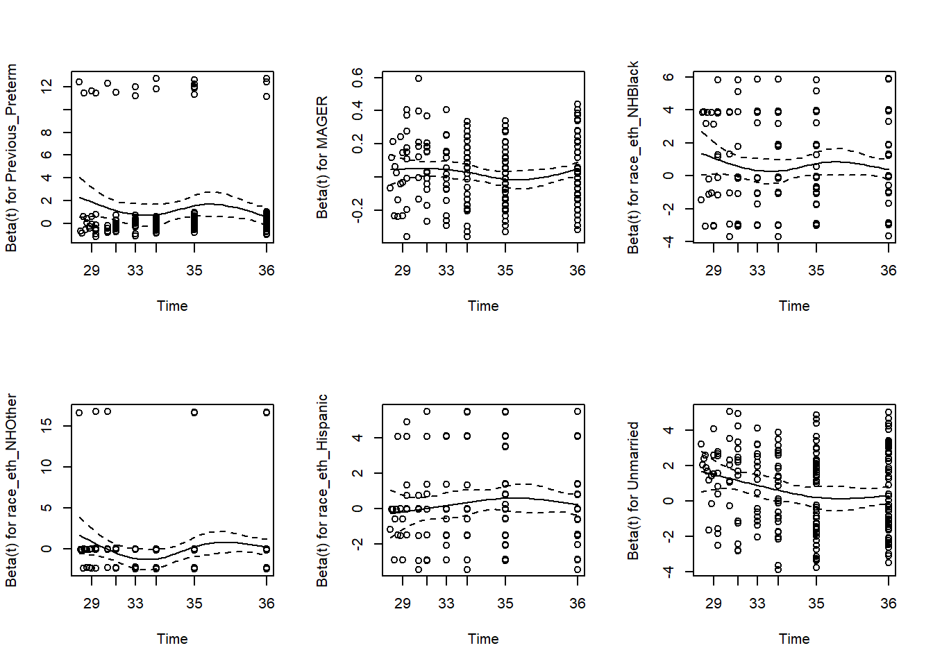
Figure 7.16: Visually assessing the proportional hazards assumption
If the null hypothesis is correct (proportional hazards), then the \(\beta\) trajectories will be close to horizontal. This provides a nice visualization for each predictor of both the magnitude of deviation from the PH assumption and the shape of the AHR trajectory. In this example, the AHR trajectories for the first five terms are relatively flat, but the trajectory for Unmarried decreases with time.
The following subsections discuss how to relax the PH assumption for a continuous predictor (using MAGER, mother’s age, for illustration even though it does not significantly violate the PH assumption in this example) and a categorical predictor (Unmarried). Two methods are covered: including an interaction between a predictor and time and stratifying by a categorical predictor.
7.16.2 Adding a time interaction for a continuous predictor
“Interacting a predictor with time” means including that predictor’s main effect plus the product of the predictor and some function of time. Which function to use can be based on the shape of the HR trajectory shown when plotting the output of cox.zph(). As mentioned previously, modeling the HR for \(X_k\) as varying linearly with time is accomplished by replacing \(\beta_k X_k\) with \(\beta_k(t) X_k\) where \(\beta_k(t) = \beta_{k_1} + \beta_{k_2} t\). Equivalently, replace \(\beta_k X_k\) with \(\beta_{k1}X_k + \beta_{k2} t X_k\). In other words, to model a linearly varying HR, add to the model an interaction between the predictor and \(t\).
We could, instead, assume a non-linear function of time. For example, modeling the HR as varying logarithmically with time corresponds to replacing \(\beta_k X_k\) with \(\beta_{k1}X_k + \beta_{k2} \ln(t) X_k\), or adding an interaction between the predictor and \(\ln(t)\). Either of these approaches, linear or non-linear, relaxes the PH assumption by replacing \(X\)’s time-invariant regression coefficient with a function of time.
Example 7.6 (continued): Relax the PH assumption for age by assuming the age effect varies linearly with time.
As mentioned above, accomplishing this requires adding, in addition to the age main effect, an interaction between age and linear time. However, we cannot add t:X to the model since “time” is the outcome – you cannot include the outcome as part of a predictor. Adding a time interaction in coxph() requires adding a special tt() function term, as well as a programming statement defining the function. To add a linear interaction with time, use the function \(tt(x,t) = x*t\).
## coxph(formula = Surv(gestage37, preterm01) ~ RF_PPTERM + MAGER +
##     MRACEHISP + DMAR, data = natality.complete)
# Re-fit the model, including tt(x,t) to add the interaction with time
cox.ex7.6.tt <- coxph(Surv(gestage37, preterm01) ~ RF_PPTERM +
MRACEHISP + DMAR +
MAGER + tt(MAGER),
data = natality.complete,
tt = function(x,t,...) x*t)
summary(cox.ex7.6.tt)$coef## coef exp(coef) se(coef) z Pr(>|z|)
## RF_PPTERMYes 1.063036 2.8951 0.236600 4.4930 0.000007024
## MRACEHISPNH Black 0.559185 1.7492 0.177545 3.1495 0.001635243
## MRACEHISPNH Other -0.073279 0.9293 0.295551 -0.2479 0.804179208
## MRACEHISPHispanic 0.259949 1.2969 0.179096 1.4514 0.146654688
## DMARUnmarried 0.584711 1.7945 0.153347 3.8130 0.000137290
## MAGER -0.068712 0.9336 0.137613 -0.4993 0.617559391
## tt(MAGER) 0.002948 1.0030 0.004039 0.7299 0.465467436## Analysis of Deviance Table (Type III tests)
##
## Response: Surv(gestage37, preterm01)
## Df Chisq Pr(>Chisq)
## RF_PPTERM 1 20.19 0.000007 ***
## MRACEHISP 3 10.80 0.01283 *
## DMAR 1 14.54 0.00014 ***
## MAGER 1 0.25 0.61756
## tt(MAGER) 1 0.53 0.46547
## ---
## Signif. codes: 0 '***' 0.001 '**' 0.01 '*' 0.05 '.' 0.1 ' ' 1As is the case with any variable involved in an interaction, you can no longer treat the main effect for MAGER as the age effect. Instead, it is the age effect at gestational age 0 weeks. The p-value for tt(MAGER) (p = .465) is a test of the interaction and also a test of the PH assumption (specifically against the alternative of a linear time interaction; cox.zph() is more general).
In the original PH model, the AHR for MAGER was \(e^{0.0313} = 1.03\). How does adding the interaction with time change this? Instead of AHR = \(e^{\beta_\textrm{MAGER}}\), we now have AHR = \(e^{\beta_\textrm{MAGER} + t*\beta_\textrm{tt(MAGER)}}\). In our example, then, the AHR for mother’s age is
\(e^{-0.0687 + 0.0029*t}\).
- At \(t = 0\) (conception), the AHR is \(e^{-0.0687} = 0.93\).
- At \(t = 30\) weeks, it is \(e^{-0.0687 + 0.0029*30} = 1.02\).
- At \(t = 35\) weeks, it is \(e^{-0.0687 + 0.0029*35} = 1.04\).
Compute the time at which the AHR is 1 using the formula \(-\beta_X / \beta_{tt(X)}\) (which is the value of \(t\) at which \(e^{\beta_X + t*\beta_{tt(X)}} = 1\)).
## MAGER
## 23.31
This implies that the direction of association changes at 23.3 weeks. If this value is not in the range of the observed event times, then the AHR is either always <1 or always >1. Figure 7.17 illustrates how the AHR changes over time.
# Range of observed event times
SUB    <- natality.complete$preterm01 == 1
TIME   <- seq(min(natality.complete$gestage37[SUB]),
              max(natality.complete$gestage37[SUB]), 1)
BETA   <- coef(cox.ex7.6.tt)["MAGER"]
BETATT <- coef(cox.ex7.6.tt)["tt(MAGER)"]
AHR    <- exp(BETA + BETATT*TIME)
plot(AHR ~ TIME, type = "l")
abline(h = 1, lty = 2, col = "darkgray")
abline(v = -1*BETA/BETATT, lty = 2, col = "darkgray")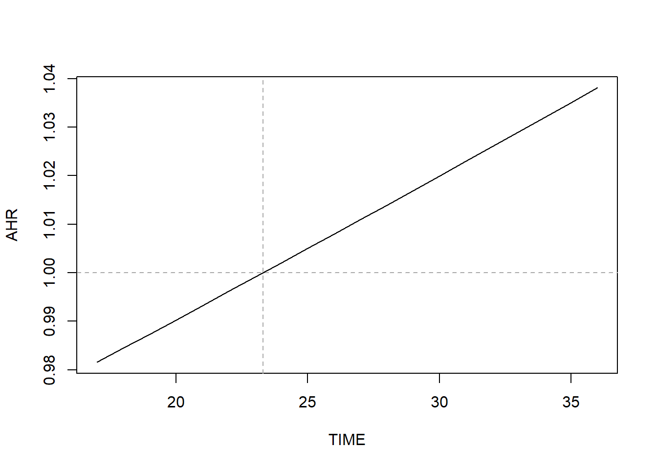
Figure 7.17: AHR varying over time when relaxing the proportional hazard assumption
In general, the AHR vs. time plot will be curved. For this continuous predictor, the curve just happens to be approximately linear over this range of weeks.
Conclusion: Based on the original PH model, those who are one year older have 3.2% greater hazard of preterm birth (AHR = 1.03; 95% CI = 1.01, 1.06; p = .009). Based on the model that relaxes the PH assumption, this difference varies over time, with younger women having greater hazard of preterm birth earlier in pregnancy and older women greater hazard later in pregnancy (because AHR <1 early, and AHR >1 late). Again, for this predictor, the PH assumption was not actually violated, but we proceeded with relaxing the assumption for illustration.
NOTE: Be careful when interpreting Figure 7.17 – it shows how the hazard ratio comparing those who differ by 1-unit in \(X\) changes over time, not how the hazard changes over time.
7.16.3 Adding a time interaction for a categorical predictor
Example 7.6 (continued): Relax the PH assumption for marital status by assuming the effect of Unmarried varies linearly with time.
The tt() function only accepts numeric predictors. We used model.matrix() in Section 7.16.1 to create the numeric indicator variable for DMAR = “Unmarried”. Since that variable is numeric, we can use it here, as well.
The code below includes the interaction with time after replacing the factor variable DMAR with its corresponding numeric indicator variable, Unmarried. In general, for a categorical predictor with \(L\) levels, replace the factor variable with the corresponding \(L - 1\) indicator variables and add a tt() term for each level that has non-proportional hazards.
# Re-fit the model, including tt(x,t) to add the interaction with time
cox.ex7.6.tt2 <- coxph(Surv(gestage37, preterm01) ~ RF_PPTERM + MAGER +
                 MRACEHISP + Unmarried + tt(Unmarried),
                 data = natality.complete,
                 tt=function(x,t,...) x*t)
summary(cox.ex7.6.tt2)$coef
## coef exp(coef) se(coef) z Pr(>|z|)
## RF_PPTERMYes 1.05525 2.8727 0.23668 4.459 0.000008253
## MAGER 0.03130 1.0318 0.01205 2.598 0.009369082
## MRACEHISPNH Black 0.55553 1.7429 0.17770 3.126 0.001770542
## MRACEHISPNH Other -0.07063 0.9318 0.29555 -0.239 0.811110305
## MRACEHISPHispanic 0.26217 1.2998 0.17914 1.464 0.143328318
## Unmarried 7.19074 1327.0797 2.22153 3.237 0.001208583
## tt(Unmarried) -0.19377 0.8238 0.06466 -2.996 0.002731143## Analysis of Deviance Table (Type III tests)
##
## Response: Surv(gestage37, preterm01)
## Df Chisq Pr(>Chisq)
## RF_PPTERM 1 19.88 0.0000083 ***
## MAGER 1 6.75 0.0094 **
## MRACEHISP 3 10.64 0.0138 *
## Unmarried 1 10.48 0.0012 **
## tt(Unmarried) 1 8.98 0.0027 **
## ---
## Signif. codes: 0 '***' 0.001 '**' 0.01 '*' 0.05 '.' 0.1 ' ' 1Just like for the continuous predictor, we can evaluate how the AHR for DMAR changes with time. In the original PH model, the AHR for DMAR (Unmarried vs. Married) was \(e^{0.5850} = 1.79\). How does adding the interaction with time change this? Instead of AHR = \(e^{\beta_\textrm{DMARUnmarried}}\), we now have AHR = \(e^{\beta_\textrm{Unmarried} + t*\beta_\textrm{tt(Unmarried)}}\). In our example, then, the AHR for mother’s age is
\(e^{7.1907 - 0.1938*t}\).
- At \(t = 0\) (conception), the AHR is \(e^{7.1907} = 1327.08\).
- At \(t = 30\) weeks, it is \(e^{7.1907 - 0.1938*30} = 3.97\).
- At \(t = 35\) weeks, it is \(e^{7.1907 - 0.1938*35} = 1.51\).
Compute the time at which the AHR is 1 using the following formula.
## Unmarried
##     37.11
Since this is beyond the range of our time variable, the AHR will never be exactly 1 and the direction of association does not change over time. Visualize how the AHR changes over time by computing it over a range of times and plotting (Figure 7.18).
SUB    <- natality.complete$preterm01 == 1
TIME   <- seq(min(natality.complete$gestage37[SUB]),
              max(natality.complete$gestage37[SUB]), 1)
BETA   <- coef(cox.ex7.6.tt2)["Unmarried"]
BETATT <- coef(cox.ex7.6.tt2)["tt(Unmarried)"]
AHR    <- exp(BETA + BETATT*TIME)
plot(AHR ~ TIME, type = "l")
abline(h = 1, lty = 2, col = "darkgray")
abline(v = -1*BETA/BETATT, lty = 2, col = "darkgray")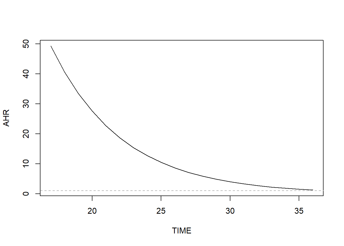
Figure 7.18: AHR varying non-linearly over time when relaxing the proportional hazard assumption
Here we clearly see the curved shape of the AHR curve. Why is the AHR so large early in pregnancy? It turns out that almost all of the earliest preterm births occurred among unmarried women. Therefore, in this dataset the hazard of preterm birth early in pregnancy is much greater for unmarried than married women.
natality.complete %>%
  filter(preterm01 == 1) %>%
  arrange(gestage37) %>%
  select(gestage37, DMAR) %>%
  slice(1:10)
## # A tibble: 10 × 2
## gestage37 DMAR
## <dbl> <fct>
## 1 17 Unmarried
## 2 20 Unmarried
## 3 23 Unmarried
## 4 24 Unmarried
## 5 25 Unmarried
## 6 26 Unmarried
## 7 27 Unmarried
## 8 27 Married
## 9 28 Unmarried
## 10 28 MarriedConclusion: Based on the original PH model, those who are unmarried have 79.5% greater hazard of preterm birth (AHR = 1.79; 95% CI = 1.33, 2.42; p <.001). Based on the model that relaxes the PH assumption, the AHR decreases with time. It is always >1 but is greater earlier in pregnancy.
NOTE: We used \(tt(x,t) = xt\) to model how the AHR changes with time. Instead, we could have used a different function of time (e.g., logarithm, polynomial, spline). Had we done so, some of the code above would need to be altered to obtain the correct plot and time at which AHR = 1.
7.16.4 Stratifying by a categorical variable
For a categorical predictor, another method of relaxing the PH assumption is to use stratification. In a stratified model, each level of the strata variable (e.g., Married, Unmarried) is assumed to have a different baseline hazard function but the same coefficients for the other predictors in the model. Because the baseline hazard functions in different strata can vary over time differently, the ratio of hazards between individuals in different strata can vary over time. While stratification removes the PH assumption for the strata variable, within levels of the strata variable PH is still assumed for the other predictors.
Example 7.6 (continued): Use stratification to relax the PH assumption for marital status.
Re-fit the model, including replacing DMAR with strata(DMAR).
NOTE: When stratifying by X, do not include X in the model, just strata(X).
cox.ex7.6.strata <- coxph(Surv(gestage37, preterm01) ~ RF_PPTERM + MAGER +
                 MRACEHISP + strata(DMAR),
                 data = natality.complete)

summary(cox.ex7.6.strata)$coef
## coef exp(coef) se(coef) z Pr(>|z|)
## RF_PPTERMYes 1.05413 2.8695 0.23670 4.4535 0.00000845
## MAGER 0.03128 1.0318 0.01205 2.5965 0.00941837
## MRACEHISPNH Black 0.55508 1.7421 0.17771 3.1236 0.00178676
## MRACEHISPNH Other -0.07071 0.9317 0.29555 -0.2393 0.81090523
## MRACEHISPHispanic 0.26203 1.2996 0.17914 1.4627 0.14355676## Analysis of Deviance Table (Type III tests)
##
## Response: Surv(gestage37, preterm01)
## Df Chisq Pr(>Chisq)
## RF_PPTERM 1 19.83 0.0000084 ***
## MAGER 1 6.74 0.0094 **
## MRACEHISP 3 10.62 0.0139 *
## ---
## Signif. codes: 0 '***' 0.001 '**' 0.01 '*' 0.05 '.' 0.1 ' ' 1The output looks very similar to an unstratified model, except that now there is no estimate of the effect of the predictor on which you stratified (there is no row for DMAR in the output above). If you want to estimate an AHR for DMAR, do not use stratification, instead include a time interaction as described previously.
Finally, re-check the PH assumption after stratification to verify that there is no remaining violation of the assumption (Figure 7.19).
# Replace factors with indicator variables
cox.ex7.6.strata.indicator <- coxph(Surv(gestage37, preterm01) ~
                   Previous_Preterm + MAGER +
                   race_eth_NHBlack + race_eth_NHOther + race_eth_Hispanic +
                   strata(DMAR),
                 data = natality.complete)

# Verify the fit is the same
summary(cox.ex7.6.strata)$coef
## coef exp(coef) se(coef) z Pr(>|z|)
## RF_PPTERMYes 1.05413 2.8695 0.23670 4.4535 0.00000845
## MAGER 0.03128 1.0318 0.01205 2.5965 0.00941837
## MRACEHISPNH Black 0.55508 1.7421 0.17771 3.1236 0.00178676
## MRACEHISPNH Other -0.07071 0.9317 0.29555 -0.2393 0.81090523
## MRACEHISPHispanic 0.26203 1.2996 0.17914 1.4627 0.14355676## coef exp(coef) se(coef) z Pr(>|z|)
## Previous_Preterm 1.05413 2.8695 0.23670 4.4535 0.00000845
## MAGER 0.03128 1.0318 0.01205 2.5965 0.00941837
## race_eth_NHBlack 0.55508 1.7421 0.17771 3.1236 0.00178676
## race_eth_NHOther -0.07071 0.9317 0.29555 -0.2393 0.81090523
## race_eth_Hispanic 0.26203 1.2996 0.17914 1.4627 0.14355676## chisq df p
## Previous_Preterm 1.71483 1 0.19
## MAGER 0.00781 1 0.93
## race_eth_NHBlack 1.48254 1 0.22
## race_eth_NHOther 0.28813 1 0.59
## race_eth_Hispanic 0.66920 1 0.41
## GLOBAL 3.41160 5 0.64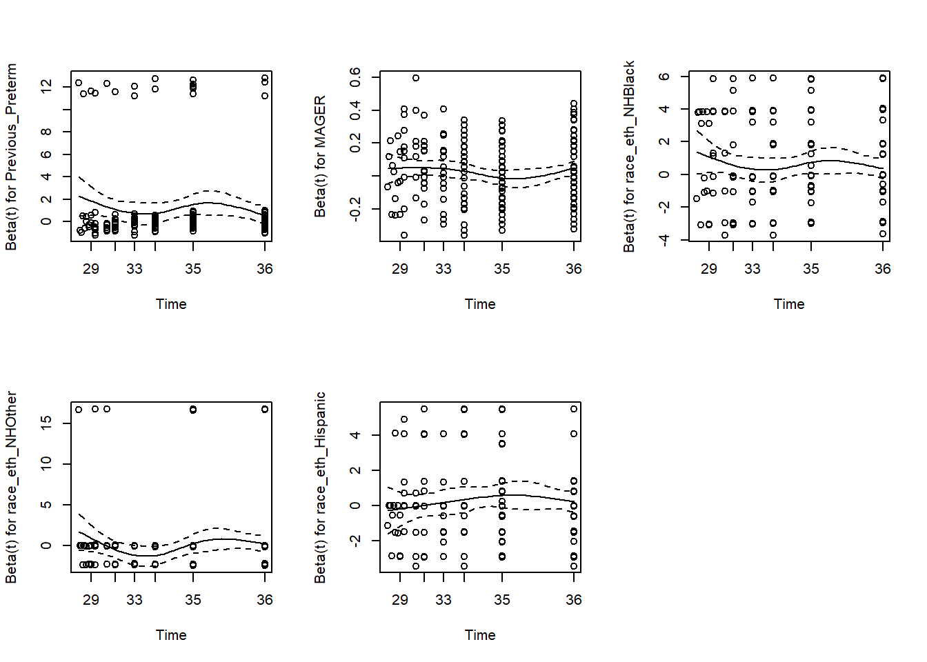
Figure 7.19: Rechecing the proportional hazards assumption