5.23 Influential observations
An influential observation is one which, when included in the dataset used to fit a model, alters the regression coefficients by a meaningful amount. A regression line attempts to provide a best fit to all the observations. Seen the other way around, each observation exerts some influence on the line, pulling the line toward itself. Observations that are extreme in the \(X\) direction are said to have high leverage – they have the potential to influence the line greatly. If you were to take a high leverage observation and change its \(Y\) value by a certain amount, the regression line would change more than if the same change were made to a low leverage observation (one near the center of the distribution of \(X\)).
However, not all high leverage observations are actually influential – those that are far from the regression line when the model is fit without them will exert more influence. Conversely, some less high leverage observations can be influential if their residuals are unusually large. The magnitude of influence is determined by the combination of leverage and magnitude of residual.
Ultimately, to assess whether an observation is actually influential, you must fit the model with and without the observation and see how the regression coefficients change. Figure 5.48 illustrates what sorts of single points are influential in an SLR with a continuous predictor. In each panel, the model is fit with and without the large solid point. The solid line is the regression line when the point is included, and the dashed line is the regression line when the point is excluded.
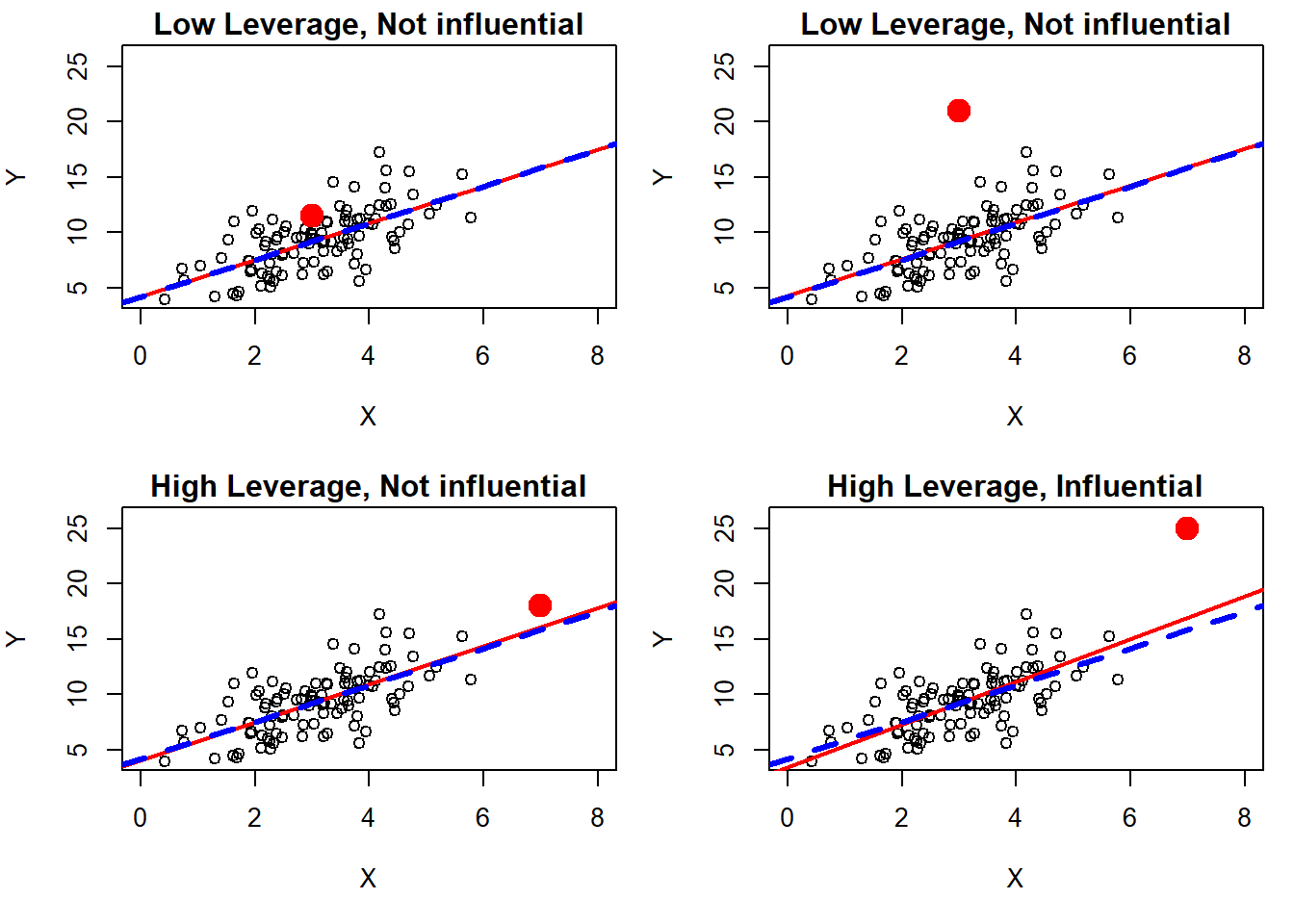
Figure 5.48: What are influential observations?
- Low leverage, Close to the line fit without the point, Not influential: In the top left panel, the solid point is close to the dashed regression line and not far from the other \(X\) values, both of which point to a lack of influence. Its lack of influence is confirmed by the fact that the regression lines are almost identical with or without this point included – the solid and dashed lines are one on top of the other.
- Low leverage, Far from the line fit without the point, Not influential: In the top right panel, despite the solid point now being very far from the dashed regression line (it is an outlier), it is not influential due to is low leverage. Again, the regression lines are almost identical with or without this point included.
- High leverage, Close to the line fit without the point, Not influential: In the bottom left panel, despite the solid point having high leverage, it is not influential since it is not far from the dashed regression line. With or without this point, the regression line remains about the same.
- High leverage, Far from the line fit without the point, Influential: In the bottom right panel, the solid point is both high leverage and far from the line fit without it, resulting in high influence. This point pulls the regression line quite a bit toward itself – when it is included, the slope increases noticeably.
5.23.1 Impact of influential observations
Influential observations pull the regression fit toward themselves. The results (predictions, parameter estimates, CIs, p-values) can be quite different with and without these cases included in the analysis. While influential observations do not necessarily violate any regression assumptions, they can cast doubt on the conclusions drawn from your sample. If a regression model is being used to inform real-life decisions, one would hope those decisions are not overly influenced by just one or a few observations.
5.23.2 Diagnosis of influential observations
If there is just one predictor, you could look at a scatterplot of \(Y\) vs. \(X\), as in Figure 5.48. With multiple predictors, however, this will not work. Regarding leverage, with multiple predictors an observation can be typical for individual predictors yet be highly unusual jointly. What makes a point high leverage is how unusual it is when considering all the predictors together. Suppose, for example, you have a model that includes the predictors height and sex. An individual may have a height that is not extreme when just looking at height, but given sex it might be extreme (e.g., males are taller than females on average, so a very tall female or a very short male may be an unusual case). Fortunately, there are diagnostics that assess leverage and influence no matter how many predictors are in the model.
- The hat value measures how far an observation’s predictors, taken together, are from those of other observations. Observations with large hat values have high leverage and are potentially (but not necessarily) influential. There is no objective cutoff above which a hat value is considered “large”. Instead, look for observations with hat values that are much larger than those of the other observations.
- Cook’s distance measures, for each observation, the difference in all the regression coefficient estimates taken together when fitting the model with and without that observation (Cook, R. D. 1977), providing a measure of global influence. There is no objective cutoff value above which a Cook’s distance is considered “large”. Instead, look for observations with Cook’s distances that are much larger than those of the other observations.
- Standardized DFBetas measure, for each observation, the standardized difference in individual regression coefficient estimates when fitting the model with and without that observation, providing a measure of influence on each coefficient. When we discuss sensitivity analyses in Section 5.26, we will see what happens to the model fit when we remove a group of observations, but DFBetas can tell us what happens when we remove each observation one-at-a-time. Standardized DFBetas can be compared to a cutoff value, with 0.2 suggested as a reasonable cutoff (Harrell 2015, p504).
Example 5.1 (continued): Look for influential observations in the model with the transformed outcome. First, look at the Studentized residuals and hat values to see if any observations are both outliers and high leverage (as these are the most potentially influential). Then look at the Cook’s distance and DFBetas to assess actual influence.
Use car::influenceIndexPlot() (Fox, Weisberg, and Price 2024; Fox and Weisberg 2019) to visualize the Studentized residuals, hat values, and Cook’s distance, as shown in Figures 5.49, 5.50, and 5.51, respectively.
car::influenceIndexPlot(fit.ex5.1.trans, vars = "Studentized",
                        id=F, main = "Studentized Residuals")

car::influenceIndexPlot(fit.ex5.1.trans, vars = "hat",
                        id=F, main = "Leverage (hat values)")

car::influenceIndexPlot(fit.ex5.1.trans, vars = "Cook",
                        id=F, main = "Cook's distance")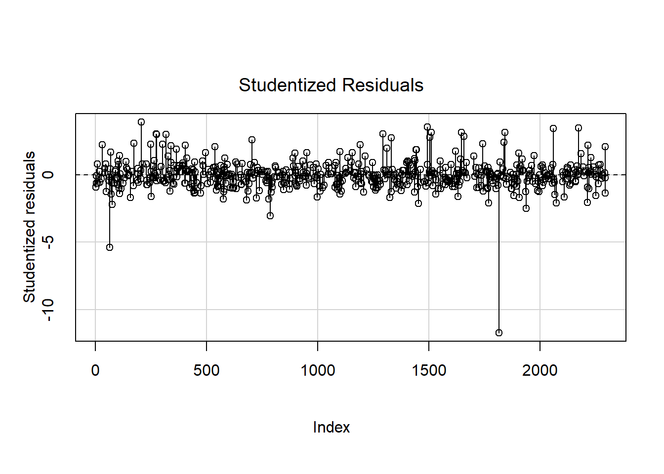
Figure 5.49: Studentized residuals
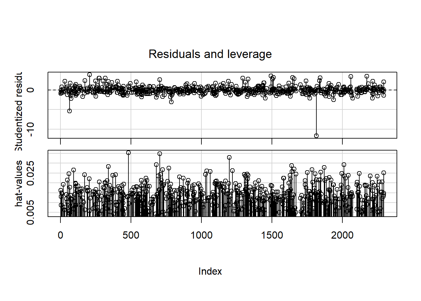
Figure 5.50: Hat values
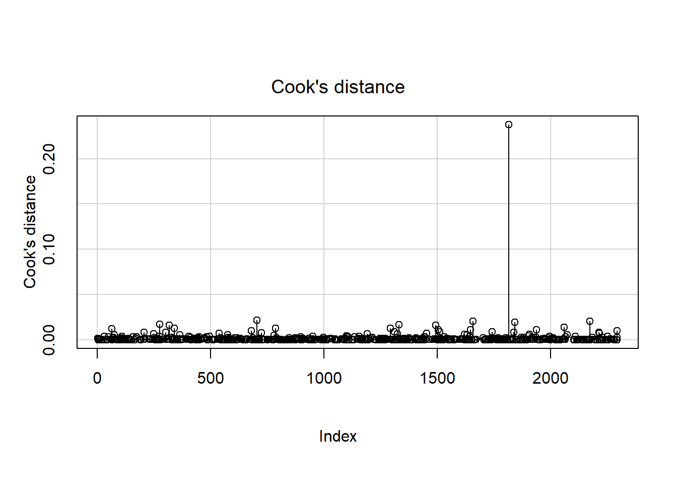
Figure 5.51: Cook’s distance
The points are plotted from left to right in the order they appear in the dataset, so their horizontal locations are not relevant. There appear to be a few hat values that stand out (Figure 5.50), indicating there are a few high leverage observations. However, those observations do not also have large residuals (Figure 5.49), so they do not actually exert much influence, as seen in their relatively small Cook’s distances. The one observation with a very large negative residual, however, has enough leverage that it has a relatively large Cook’s distance (Figure 5.51). It is the combination of leverage and being an outlier that results in high influence.
To compute these statistics directly, use the following functions.
Cook’s distance above identified one observation that highly influences the regression coefficients collectively. Next, use standardized DFBetas to assess influence on each regression coefficient individually, as shown in Figure 5.52 (only shown for a few of the predictors).
# Compute DFBETAS
DFBETAS <- dfbetas(fit.ex5.1.trans)
# Check the spelling of the terms and enter them accordingly
# in each plot() call below
# colnames(DFBETAS)
par(mfrow=c(2,3))
plot(DFBETAS[, "(Intercept)"], main="Intercept", ylab="")
abline(h = c(-0.2, 0.2), lty = 2)
plot(DFBETAS[, "BMXWAIST"], main="WC", ylab="")
abline(h = c(-0.2, 0.2), lty = 2)
plot(DFBETAS[, "smokerPast"], main="Past", ylab="")
abline(h = c(-0.2, 0.2), lty = 2)
plot(DFBETAS[, "smokerCurrent"], main="Current", ylab="")
abline(h = c(-0.2, 0.2), lty = 2)
plot(DFBETAS[, "RIDAGEYR"], main="Age", ylab="")
abline(h = c(-0.2, 0.2), lty = 2)
plot(DFBETAS[, "RIAGENDRFemale"], main="Female", ylab="")
abline(h = c(-0.2, 0.2), lty = 2)
plot(DFBETAS[, "race_ethNon-Hispanic White"], main="NHW", ylab="")
abline(h = c(-0.2, 0.2), lty = 2)
plot(DFBETAS[, "race_ethNon-Hispanic Black"], main="NHB", ylab="")
abline(h = c(-0.2, 0.2), lty = 2)
plot(DFBETAS[, "race_ethNon-Hispanic Other"], main="NHO", ylab="")
abline(h = c(-0.2, 0.2), lty = 2)
plot(DFBETAS[, "income$25,000 to <$55,000"], main="$25-$54", ylab="")
abline(h = c(-0.2, 0.2), lty = 2)
plot(DFBETAS[, "income$55,000+"], main="$55+", ylab="")
abline(h = c(-0.2, 0.2), lty = 2)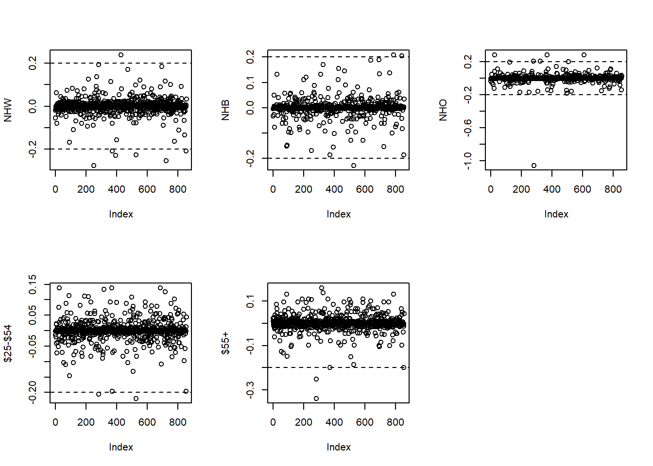
Figure 5.52: Standardized DFBetas
Each DFBeta plot shows, on the vertical axis, how much that predictor’s regression coefficient changes when an observation is removed, on a standardized scale. A few points appear to have large standardized DFBetas (greater in absolute value than 0.2, indicating removal of that observation would change that \(\beta\) by more than 0.2 standard deviations).
5.23.3 Potential solutions for influential observations
- Predictor transformation: A highly skewed \(X\) distribution can lead to high leverage for points at the extreme. A transformation (e.g., logarithm, square root, inverse) may solve this problem.
- Outcome transformation: If the \(Y\) distribution is very skewed, that can lead to large residuals. A transformation may solve this problem.
- Perform a sensitivity analysis: Fit the model with and without the influential observations and see what changes (see Section 5.26). If a point is influential based on the diagnostics, that alone does not justify its removal. As with outliers, never simply remove observations from the data just because they might be problematic. Instead, do the analysis with and without them and state the differences in any discussion of the results.