7.25 Exercises
True or false? Time-to-event data can easily be handled using linear regression.
Name two reasons why logistic regression may be inappropriate for time-to-event data.
During an infectious disease pandemic, researchers follow vaccinated individuals for 1 year post-vaccination and compare the outcome “time to infection” between groups receiving two different vaccines. What type of outcome is this and what regression method would be appropriate for this outcome?
In Exercise 3, suppose the researchers only know whether or not each individual experienced the disease during the year after vaccination. What type of outcome is this and what regression method would be appropriate for this outcome?
In Exercise 3, suppose some individuals who have not yet experienced infection are lost to follow-up prior to 1 year. What kind (right, left, or interval) and mechanism (Type I, Type II, or random) of censoring is this? Suppose some individuals have not yet experienced infection when the study ends at 1 year. What kind and mechanism of censoring is this?
During an infectious disease pandemic, researchers follow vaccinated individuals post-vaccination and record the outcome “time to infection”. They stop the study after 100 individuals are infected. For individuals who never experience infection, what kind and mechanism of censoring is this?
A retrospective chart review is used to identify patients in a psychiatric clinic who received one of two different treatments for depression and the first visit at which treatment was started (the index visit). Patients were seen every 6 months following the index visit. Follow-up charts were reviewed to determine when each patient first no longer met criteria for depression. For the outcome “time to remission”, are the times censored and, if so, with what kind of censoring?
Suppose you want to carry out a hypothesis test in which the null hypothesis is that survival is the same for three groups of individuals. Name two methods of testing this hypothesis.
In the previous exercise, suppose you wanted to carry out the test after adjusting for confounding due to other variables. Would both methods still work?
After fitting a Cox regression model, what two assumptions should you check, and what alternatives are possible if each assumption is not met?
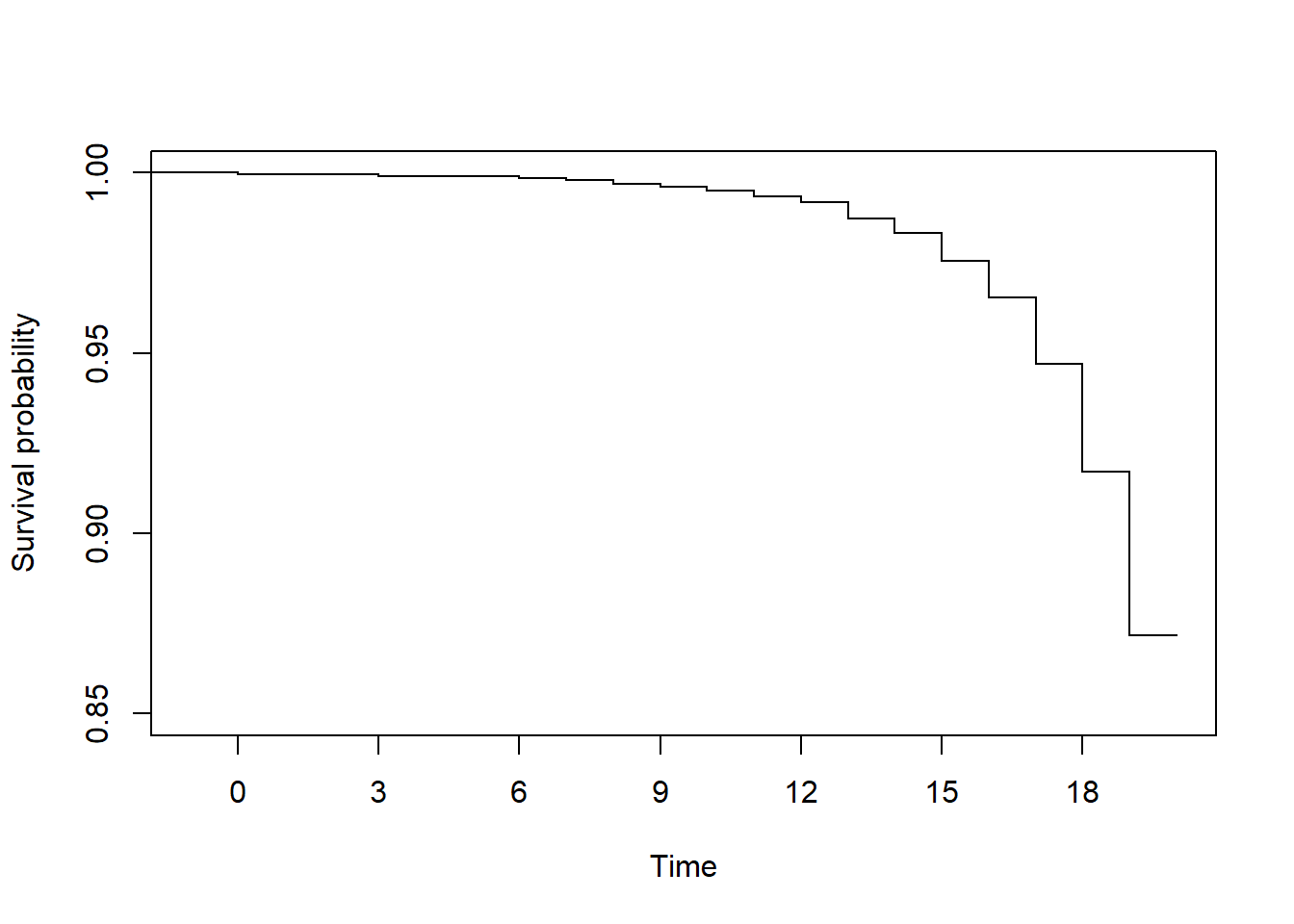
In the survival function below, approximately what is S(18)?
For Exercises 12-17, use the Digitalis teaching dataset (dig_rmph.rData, see Appendix A.6) to answer questions related to the time to first hospitalization for any cardiovascular disease (CVD) cause (worsening heart failure, arrythmia, Digoxin toxicity, MI, unstable angina, stroke, coronary revascularization, cardiac transplantation, or other cardiovascular event) (CVDDAYS = days from randomization to first CVD hospitalization; CVD = event indicator).
Check that the time and event indicator variables are in the correct format. If not, modify them so that they are.
Compute the Kaplan-Meier estimate of “survival” (in this case, survival is not yet being hospitalized for a CVD event) and answer the following questions.
- How many are in the risk set at randomization?
- How many CVD hospitalizations occurred in total?
- How many CVD hospitalizations occurred exactly 10 days after randomization?
- What is the estimated survival probability (probability of not yet being hospitalized for a CVD event) and 95% confidence interval 15 days after randomization?
- What is the probability of CVD hospitalization any time up to and including 500 days?
- What is the probability of CVD hospitalization strictly between 500 and 750 days after randomization?
Plot the survival function, adjusting the X and Y axes to make the curve easy to read and removing the marking of censored times (there are a lot so they clutter up the curve).
Plot the hazard function. Based on the shape of the hazard function, describe how the instantaneous risk (hazard) of CVD hospitalization changes over time.
What is the median (and 95% CI) days to CVD hospitalization?
Compute the Kaplan-Meier estimates of survival comparing treatment groups (
TRTMT) and answer the following questions.
- Which group has an earlier median time to CVD hospitalization?
- Plot the survival and hazard curves comparing treatment groups. Which treatment (placebo or Digoxin) seems to be more effective in preventing CVD hospitalization?
- Is the difference between the survival functions statistically significant?
For Exercises 18 and 19, use the NHANES examination subset teaching dataset (nhanes1718_adult_exam_sub_rmph.Rdata, see Appendix A.1) to answer questions about the association between income (income) and age when first told has asthma (MCQ025) (the event indicator is MCQ010 – “Ever been told you have asthma”).
- Do the following:
- Check that the time and event indicator variables are in the correct format. If not, modify them so that they are. Hint: For the event indicator, name the new variable “asthma”.
- “Age when first had asthma” is missing for those who have never been told they have asthma. For a time-to-event analysis, we want those who have never been told they have asthma to have a censored time. It makes sense, in this case, to set their censored “age when first had asthma” to their current age (their event indicator is already 0, so we do not need to change that). Use the following code to accomplish this (assuming your dataset name is
nhanes).
# Create a copy of the age variable
nhanes$asthma_age <- nhanes$MCQ025

# Subset on asthma = 0 and replace the missing asthma ages with current age

# SUB <- nhanes$asthma == 0
# nhanes$asthma_age[SUB] <- nhanes$RIDAGEYR[SUB]
# # Error in nhanes$asthma_age[nhanes$asthma == 0] <- nhanes$RIDAGEYR :
# #   NAs are not allowed in subscripted assignments
# The above error is due to the fact that nhanes$asthma is sometimes missing.
# When subsetting on a logical vector, you have to exclude the missing values.

# Add complete.cases() to the logic
SUB <- complete.cases(nhanes$asthma) & nhanes$asthma == 0

# Use [SUB] on both sides so the number of obs you are changing on the
# left-hand side-is equal to the number of obs you are replacing them with
# from the right hand side
nhanes$asthma_age[SUB] <- nhanes$RIDAGEYR[SUB]

# Check
# For !SUB, these should be the same
summary(nhanes$MCQ025[!SUB])
summary(nhanes$asthma_age[!SUB])
summary(nhanes$MCQ025[!SUB] - nhanes$asthma_age[!SUB])
# For SUB, this is all missing
summary(nhanes$MCQ025[SUB])
# and these should be the same
summary(nhanes$asthma_age[SUB])
summary(nhanes$RIDAGEYR[SUB])
summary(nhanes$asthma_age[SUB] - nhanes$RIDAGEYR[SUB])- Use Cox regression to test the association between income and time to asthma. Is the association statistically significant?
- Ignoring the overall statistical significance or lack thereof, compare the lower, middle, and upper income groups. Report the HR, 95% CI, and p-value for each of the three pairwise comparisons, along with an interpretation of each HR. Based on these results, what is the direction of association?
- Even if the overall association were statistically significant, it would not necessarily imply a causal relationship (greater income –> less chance of developing asthma). Income here is current income, whereas the asthma variable reflects being told sometime in the past that one has asthma. Give a possible alternative explanation for the observed association.
- Using the same dataset from the previous exercise, test the association between body mass index (BMXBMI) and time to asthma. Answer the question, report the HR, 95% confidence interval, and p-value, and interpret the HR, both for a 1-unit difference in BMI and for a 5-unit difference.
For Exercises 20 and 21, use the Digitalis teaching dataset that you created in Exercise 12.
After adjusting for age
(AGE), sex(SEX), minority status(RACE), body mass index(BMI), and systolic blood pressure (SYSBP), is the cause of congestive heart failure (chfcause) associated with time to first hospitalization for any CVD cause?CVDDAYSis the time variable and the event indicator is the modified version ofCVDyou created in Exercise 12. Answer the question, report the adjusted HRs (AHRs), 95% confidence intervals, and p-values comparing each non-reference cause to the reference level. Order the causes from least to greatest hazard of hospitalization for CVD.Using the model from the previous exercise, what is the predicted probability (and its standard error and 95% confidence interval) of not yet experiencing a CVD hospitalization 100 days post-randomization for a patient with ischemic cause of CHF, who is age 45 years, male, minority, has a BMI of 35 kg/m2, and has a systolic blood pressure of 140 mmHg?
For the patient described in the previous exercise, what is their hazard relative to a reference individual with categorical predictors at their reference level and continuous predictors at the sample mean? Report the AHR and its standard error. Does this patient have more or less hazard of CVD hospitalization than the reference patient?
For the patient described in the previous exercise, what is their hazard relative to a reference individual with categorical predictors at their reference level and continuous predictors set to 0? Report the AHR and its standard error. Why is this not a valid prediction? Compared to the predicted AHR in the previous exercise (which was valid), this AHR is not very different. Why would this invalid prediction not be very different from a valid prediction for this particular model?
Using the model from the previous exercises, plot the survival functions from the day after randomization (time = 1) to 1781 days for the four CHF cause groups. Assume the other variables are equal to that of the patient for whom you predicted the hazard in the previous exercises.
You would like to test the association between the cause of congestive heart failure (
chfcause) and time to coronary revascularization (CREV= event indicator,CREVDAYS= time to event) AMONG FEMALES, adjusted for age (AGE), minority status (RACE), body mass index (BMI), and systolic blood pressure (SYSBP). Knowing this outcome is somewhat rare, you decide to check for separation. Check for separation, resolve any issues, and fit the model to answer the research question. How did separation affect your ability to answer the research question?
For Exercises 26-28, use the teaching dataset based on the Framingham Heart Study (fram_time_invar_rmph.rData, see Appendix A.6).
Does the association between time to angina pectoris (chest pain) (
TIMEAP= time variable,ANGINA= event indicator) and the age of the participant at enrollment (AGE) differ between male and female patients (SEX)? Answer the question, including the appropriate p-value. Estimate the HR, 95% CI, and p-value for age at each level of sex, and interpret the results.In the model you fit in the previous exercise, is sex significantly associated with the outcome?
Using the full model from the previous exercises, for each level of sex, create a plot that compares the survival functions between individuals age 40, 50, and 60 years and interpret the results.
For Exercises 29 and 30, use the teaching dataset based on the Framingham Heart Study that contains time-varying predictors for the outcome death (fram_tv_death_rmph.rData, see Appendix A.6). The (START, STOP] variables are tstart and tstop and the event indicator is DEATH.
Is there an association between smoking status (
CURSMOKE) and time to death, adjusted for baseline age (AGE), sex (SEX), and education (EDUC)? Answer the question and report the adjusted hazard ratio (AHR), 95% confidence interval, p-value, and interpret the AHR. Also, which of the confounders were statistically significant?The dataset
fram_tv_death_rmph.rDatadiffers from the datasetfram_time_invar_rmph.rDatain that the former is set up using the (START, STOP] syntax in order to accommodate time-varying predictors. For analyses that involve only time-invariant predictors, you can use either dataset.
Do the following:
- Examine each dataset by looking at the rows of data for
RANDID6238 and 10552. (Hint: Use a filter statement.) Select the variables that are needed for the model fitting. For the time-varying dataset, also include the variable systolic blood pressure (SYSBP). How are the two datasets structured differently? - Fit a Cox regression model using each dataset to test the association between time to death and baseline age (
AGE), sex (SEX), and education (EDUC). For the time-varying dataset, usetstartandtstopas the time variables. For the time-invariant dataset, useTIMEDTH. For both, the event indicator isDEATH. You should get the same fit for both datasets. Had there been any time-varying predictors in the model, you would not have been able to use the time-invariant dataset because it only has one row per person.
For Exercises 31-36, use the Digitalis teaching dataset that you created in Exercise 12.
Numerically and visually assess the proportional hazards assumption for the predictors in the model you fit in Exercise 20. Hint: If the lines are difficult to see, use
lwd=3andcol="red"inside your call toplot()to make the lines stand out. If the scale is too small, use theylimoption to zoom in. For example,ylim = c(-1, 1).Continuing the previous exercise, if there is a variable that violates the proportional hazards assumption, add a time interaction and re-fit the model. Compute the time at which the AHR is 1 and plot the AHR vs. time. Interpret the results.
Instead of using a time interaction as in the previous exercise, relax the proportional hazards assumption using stratification. Re-fit the model and re-check the PH assumption. Any remaining problems?
Check the linearity assumption for the continuous predictors for the model you fit in Exercise 20 (before relaxing the proportional hazards assumption). Any serious problems? Hint: Do not worry about non-linearities that are in areas with just a few points; those are just artifacts of smoothing.
Check for outliers for the model you fit in Exercise 20 (before relaxing the proportional hazards assumption). Which individual has the largest positive residual? Examine this individual’s predictor values and the output of the model and explain why this individual has the largest residual.
Check for influential observations for the model you fit in Exercise 20 (before relaxing the proportional hazards assumption).
You are designing a study for which you wish to fit a Cox regression model with four predictors. Assuming the proportion of events (non-censored event times) is expected to be 0.23, what is the minimum sample size you need to avoid overfitting? What if the proportion of events is expected to be 0.10? What if the proportion of events is expected to be 0.80? What can you say about the relationship between the expected proportion of events and the minimum sample size for a given number of predictors?
Suppose you have a dataset with \(n = 581\) observations. In order to avoid overfitting, what is the maximum number of predictors you should include in a Cox regression model if the observed number of non-censored event times is 20, 100, or 300? What can you say about the relationship between the observed number of non-censored events and the number of predictors for a given sample size?