5.20 Interpreting a model with a transformed outcome
If the outcome has been transformed using a non-linear transformation such as a Box-Cox transformation or one of its special cases, then the relationships between the outcome and predictor based on the output of the regression model should be interpreted on the transformed scale, not the original scale. For example, in the final model we fit in Example 5.1, the regression coefficients are as follows:
##                            Estimate Std. Error  t value Pr(>|t|)
## (Intercept)                  0.5874     0.0025 235.3593   0.0000
## BMXWAIST                     0.0002     0.0000   9.7339   0.0000
## smokerPast                   0.0012     0.0008   1.4326   0.1523
## smokerCurrent               -0.0001     0.0010  -0.0764   0.9391
## RIDAGEYR                     0.0002     0.0000   9.7597   0.0000
## RIAGENDRFemale              -0.0031     0.0007  -4.4107   0.0000
## race_ethNon-Hispanic White  -0.0030     0.0010  -3.0713   0.0022
## race_ethNon-Hispanic Black  -0.0017     0.0013  -1.3146   0.1890
## race_ethNon-Hispanic Other  -0.0005     0.0014  -0.3178   0.7507
## income$25,000 to <$55,000    0.0004     0.0011   0.3809   0.7034
## income$55,000+              -0.0001     0.0010  -0.0679   0.9459
We conclude that waist circumference is positively associated with transformed fasting glucose and that a 1-unit difference in waist circumference is associated with a 0.0003 unit difference in mean \(-FG^{-1.5}\), not with a 0.0003 difference in mean fasting glucose (mmol/L) on the original scale.
This relationship holds no matter the value of waist circumference – that is what it means to have a linear relationship. However, on the original scale of FG (mmol/L), the relationship is non-linear, as illustrated in the right-hand panel of Figure 5.44. On the original scale, the effect of waist circumference on fasting glucose depends on the value of waist circumference – at lower levels the effect is less and at greater levels the effect is greater.
Note: Back-transforming using the inverse of the outcome transformation does not lead to a valid estimate of the mean outcome on the original scale. However, if the assumptions of the linear regression model are met on the transformed scale, then the mean transformed outcome is equal to the median transformed outcome, and the back-transformed median is the estimated median on the original scale (Harrell 2015, 391).
# Vector of WC values at which to predict
X    <- seq(min(nhanesf.complete$BMXWAIST),
            max(nhanesf.complete$BMXWAIST))

# Estimate mean outcome for these WC values
# Assume other predictors are at their mean
# or reference level
PRED <- predict(fit.ex5.1.trans,
                data.frame(BMXWAIST = X,
                           smoker   = "Never",
                           RIDAGEYR = mean(nhanesf.complete$RIDAGEYR),
                           RIAGENDR = "Male",
                           race_eth = "Hispanic",
                           income   = "<$25,000"))

# Plot on transformed scale
par(mfrow = c(1, 2))
plot(PRED ~ X, type = "l",
     ylab = "Mean Transformed Fasting Glucose",
     xlab = "Waist Circumference (cm)",
     main = "Transformed Outcome")

# PRED = (LBDGLUSI^LAMBDA - 1) / LAMBDA
# Back-transform to the original scale
FG <- (1 + LAMBDA*PRED)^(1/LAMBDA)
# Plot on original scale
plot(FG ~ X, type = "l",
     ylab = "Median Fasting Glucose (mmol/L)",
     xlab = "Waist Circumference (cm)",
     main = "Original Scale")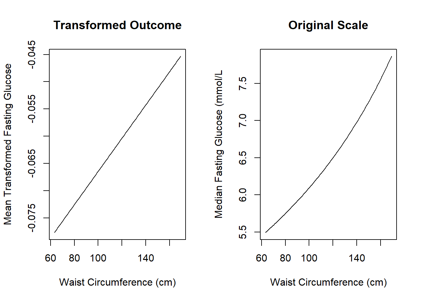
Figure 5.44: Interpreting a transformed outcome
This is similar to the effect of including a polynomial transformation of a predictor (see Section 4.8) – the relationship between the outcome and the predictor, on the original scale, becomes non-linear.