6.16 Goodness-of-fit
Since a binary outcome can only take on two possible values, numerically represented as 1 for the condition of interest and 0 otherwise, how close individual predicted values are to observed values is not a great indication of goodness-of-fit. The logistic regression curve does not actually go through most of the 1s and 0s (see Figure 6.2). However, within a group of individuals, we can expect a good-fitting model to produce predicted probabilities that are similar to the observed proportion of \(Y = 1\) values within that group.
6.16.1 Hosmer-Lemeshow test
The Hosmer-Lemeshow test (Hosmer and Lemeshow 2000) (HL test) quantifies this expectation by splitting the data into ten groups based on their predicted probabilities and then, within groups, comparing the observed and expected proportions. The first group is the 10% of observations with the lowest predicted probabilities, the second is the 10% with the next lowest, and so on. If the model fits well, we expect the observed proportions of \(Y = 1\) in these groups to be similar to their within-group average predicted probabilities.
The HL test compares the observed to expected within each group and sums over groups to obtain a statistic that has a chi-square distribution. If the overall deviation is large, then the statistic will be large and the p-value will be small, resulting in rejection of the null hypothesis that the data arise from the specified model. In other words, a large p-value indicates a good fit and a small p-value indicates a poor fit.
You can carry out the HL test in R using ResourceSelection::hoslem.test() (Lele, Keim, and Solymos 2023). The function requires you to input the outcome values (as 0s and 1s) and fitted probabilities. Extract the outcome and fitted values from a model fit using fit$y and fit$fitted.values. Using fit$y is safer than extracting the outcome from the dataset (e.g., nsduh$mj_lifetime) – if there are missing values, the outcome extracted from the dataset will have a different length than the fitted values.
Example 6.3 (continued): Assess goodness-of-fit for the model with an interaction.
HL <- ResourceSelection::hoslem.test(fit.ex6.3.int$y,
                                     fit.ex6.3.int$fitted.values)

# View the test
HL
##
## Hosmer and Lemeshow goodness of fit (GOF) test
##
## data: fit.ex6.3.int$y, fit.ex6.3.int$fitted.values
## X-squared = 2.9, df = 8, p-value = 0.9##
## cutyhat y0 y1
## [0.000118,0.24] 76 11
## (0.24,0.379] 56 28
## (0.379,0.495] 50 34
## (0.495,0.563] 37 45
## (0.563,0.635] 40 53
## (0.635,0.695] 24 53
## (0.695,0.74] 25 59
## (0.74,0.795] 15 68
## (0.795,0.855] 15 70
## (0.855,0.99] 8 76##
## cutyhat yhat0 yhat1
## [0.000118,0.24] 76.771 10.229
## (0.24,0.379] 57.228 26.772
## (0.379,0.495] 46.307 37.693
## (0.495,0.563] 38.208 43.792
## (0.563,0.635] 36.395 56.605
## (0.635,0.695] 25.522 51.478
## (0.695,0.74] 23.549 60.451
## (0.74,0.795] 19.160 63.840
## (0.795,0.855] 14.828 70.172
## (0.855,0.99] 8.032 75.968In the output above, we see that the test split the observations into ten groups. Although the sample sizes in the groups are not shown, they are approximately equal (to verify this, sum each row in the observed table). Within each group, the HL test compares the observed frequencies to the predicted, combines this information into a chi-square test statistic, and computes a p-value as the probability of observing a chi-square value at least as large under the null hypothesis of a perfect fit.
Conclusion: In this example, p > .05 so we do not reject the null hypothesis of a perfect fit, and we conclude the fit is adequate.
NOTE: The HL test with the default of ten bins may fail (resulting in a p-value of NA) in a model with few predictors, as there will not be enough unique fitted values to create ten bins. You can reduce the number of bins using the g option.
##
##  Hosmer and Lemeshow goodness of fit (GOF) test
##
## data:  fit.ex6.3.int$y, fit.ex6.3.int$fitted.values
## X-squared = 3.1, df = 7, p-value = 0.9
6.16.2 Calibration plot
P-values depend heavily on the sample size. Therefore, we must be careful since the HL test may lack power to detect a poor fit in a small sample (and we would therefore incorrectly conclude the fit is good) and may detect even minor deviations in a large sample (and we would therefore incorrectly conclude the fit is poor). It is helpful, along with looking at the HL test p-value, to create a calibration plot (Harrell 2015; Steyerberg 2009) to visualize the relationship between the observed and expected values. The calibration.plot() function (in Functions_rmph.R which you loaded at the beginning of this chapter) creates a calibration plot corresponding to the HL test, and displays the HL test p-value on the plot.
Example 6.3 (continued): Use a calibration plot to visualize goodness-of-fit for the model with an interaction.
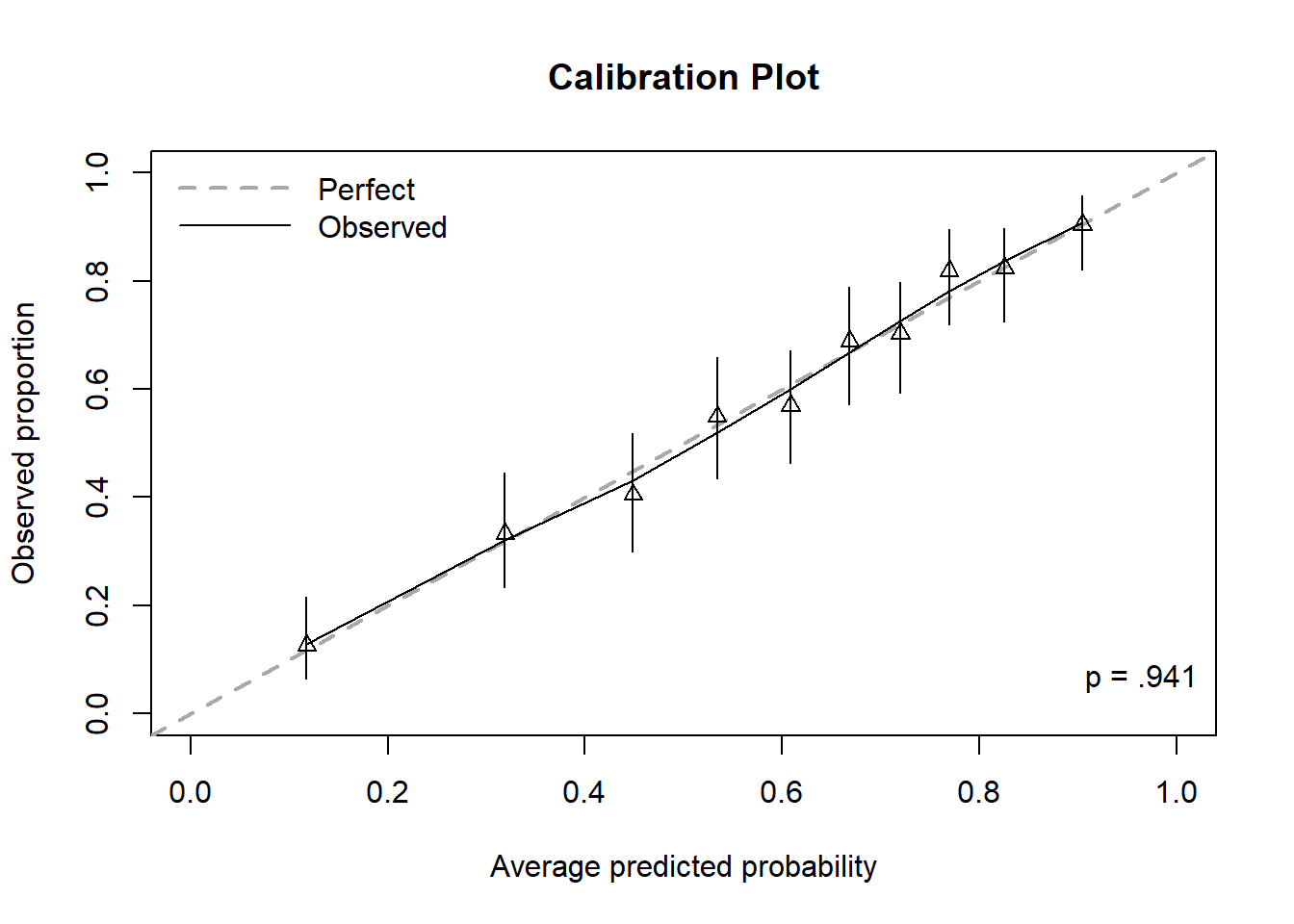
Figure 6.9: Calibration plot for a logistic regression, including Hosmer-Lemeshow test p-value
In Figure 6.9, the first triangle is plotted at (x, y) where x = the average predicted probability among those in the first bin and y = the observed proportion of outcomes in the first bin (11 / (11 + 76) = 0.126). The first triangle is very close to the 45\(^\circ\) line indicating the model is predicting probabilities in the first bin that are, on average, close to the observed proportion of outcomes. The remaining triangles are plotted similarly, one for each bin. Perfect calibration would be indicated by all the triangles falling exactly on the 45\(^\circ\) line.
The vertical lines going through each triangle represent 95% CIs for the population proportions. The solid “Observed” curve is a smoother and since, in this example, it pretty much tracks along the 45\(^\circ\) line, the calibration of this model is very good, on average.
Plotting the same plot along with the bin boundaries and the observed values makes it easier to understand where this plot is coming from (Figure 6.10).
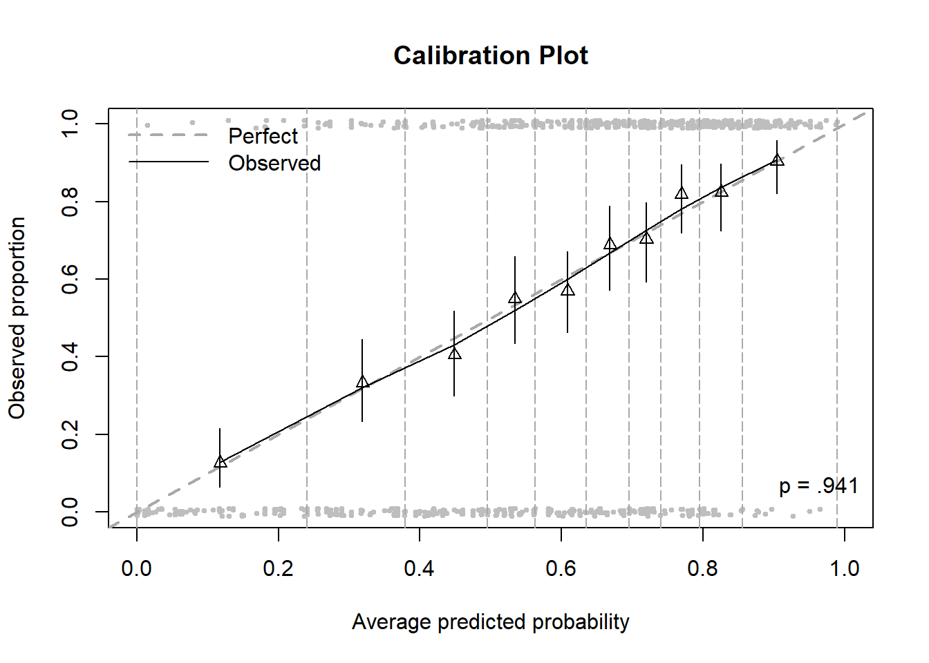
Figure 6.10: Calibration plot including bins and points
The gray points (individual observations) are plotted left to right in order from lowest to highest predicted probability, those with \(Y = 1\) at the top and those with \(Y = 0\) at the bottom (jittered to make it easier to see how many there are). The vertical dashed lines are the bin boundaries and, by design, each bin has about the same number of observations.
Conclusion: The calibration plot confirms the conclusion of the HL test, that the model fits this data well.
Rare outcome
If you are modeling a rare outcome, some adjustments can be made to the calibration plot to zoom in on a smaller range of probabilities.
Example 6.4 (continued): Visualize goodness-of-fit for the model for lifetime heroin use that we obtained after resolving separation by collapsing age categories.
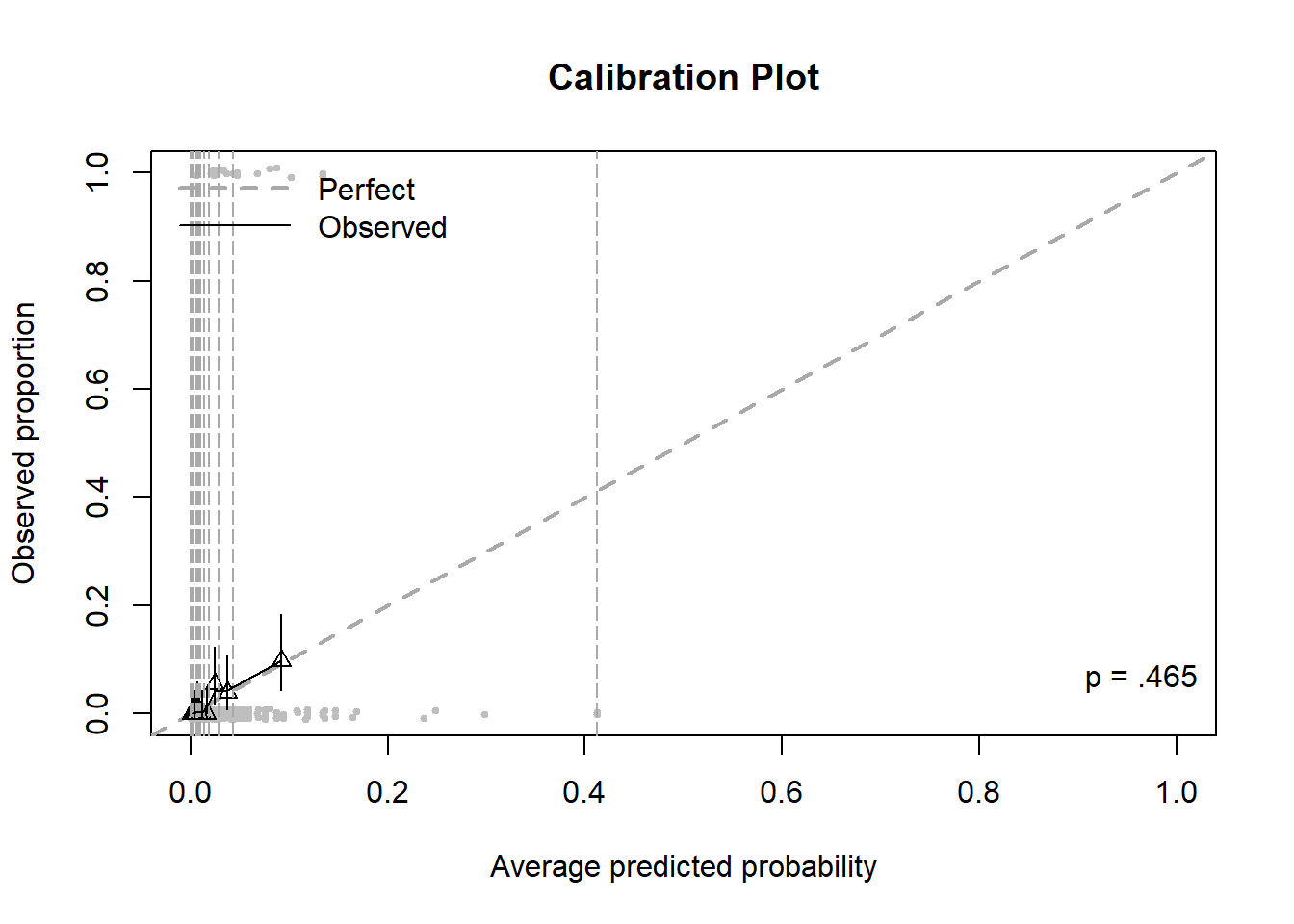
Figure 6.11: Calibration plot for a logistic regression with a rare outcome, before zooming
The outcome lifetime heroin use is more rare than lifetime marijuana use. Thus, there are very few large predicted probabilities. The result is a plot that is hard to read due to having one large bin for the largest probabilities and all the other bins being squished together (Figure 6.11). The calibration.plot() function has options that can solve this problem by zooming in on the points: zoom, zoom.x, or zoom.y, each of which can be FALSE, the default, TRUE to automatically zoom, or a vector of limits to customize the amount of zooming.
Figure 6.12 displays the calibration plot for the prediction of lifetime heroin use after zooming in on the x and y axes (so much so that the bin furthest to the right is cut out altogether). The model does not appear to be well calibrated since many triangles seem “far” from the diagonal. However, be careful when zooming in, as even small differences between observed proportions and predicted probabilities can appear large. This does illustrate, however, the difficulty in estimating rare probabilities – a very large sample size is needed to obtain reliable estimates of very small probabilities.
Whether this model fits well or not comes down to how important it is to estimate the smallest probabilities well. If knowing that a probability is “small” is good enough, then this model may be considered to fit well. The first seven bins all have CIs that are bounded above by 0.06. So, while some bins have triangles “far” from the diagonal, if any distinction beyond “this probability is small” is not important, then the model is doing its job well. If, on the other hand, you really want to make distinctions between small probabilities, then perhaps it does not fit well.
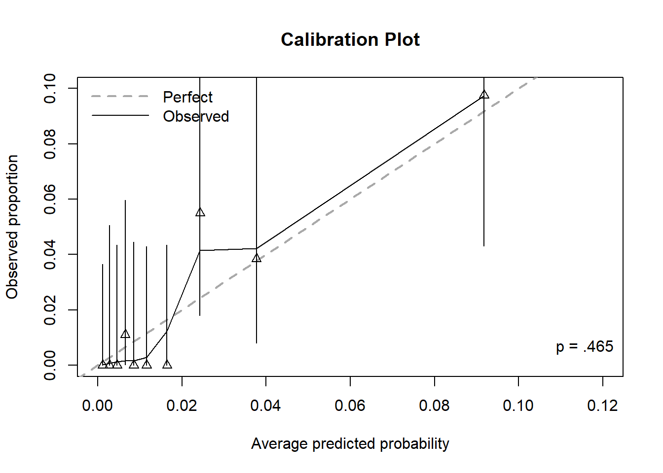
Figure 6.12: Calibration plot for a logistic regression with a rare outcome, after zooming
NOTES:
- The calibration plot with the default of ten bins may return an error in a model with few predictors, as there will not be enough unique fitted values to create ten bins. You can reduce the number of bins using the
goption (this will also then use this value ofgfor the HL test p-value that is printed on the plot). - There are some cases where
g=10works forResourceSelection::hoslem.test()but fails forcalibration.plot(). Despite not being able to create enough bins, the former ends up with one bin that is much larger than the others. If you need to use a smallergforcalibration.plot(), then also use that samegforResourceSelection::hoslem.test().
6.16.3 Relationship between the HL test p-value and the calibration plot
The null hypothesis for the HL test is that the triangles fall exactly on the diagonal in the population. If the triangles in the sample fall “close enough” to the diagonal, then the model is well calibrated. However, when using a statistical hypothesis test, what counts as “close enough” changes with the sample size.
In general, the p-value of the HL test is smaller (indicating poorer fit) when the CIs do not overlap the diagonal. Triangles far from the diagonal, an indication of a poor fit, are more likely to have CIs that do not overlap the diagonal, so this seems reasonable. However, small samples result in less precise estimates and wider CIs. Therefore, in a small sample, the triangles could be far from the diagonal but have CIs that are so wide they cross it, leading to the incorrect conclusion of a good fit. In general, goodness-of-fit tests lack power to detect poor fit in small samples.
Conversely, the p-value of the HL test is larger (indicating better fit) when the CIs do cross the diagonal. Triangles close to the diagonal, an indication of a good fit, are more likely to have CIs that overlap the diagonal, so this seems reasonable. However, large samples result in more precise estimates and narrower CIs. Therefore, in a large sample, the triangles could be close to the diagonal but have CIs that are so narrow they fail to cross it, leading to the incorrect conclusion of a poor fit. In general, goodness-of-fit tests are overly sensitive to minor deviations from perfect fit in large samples.
There are two other possibilities: triangles far from the diagonal with CIs that do not cross it (poor fit) or triangles close to the diagonal with CIs that do cross it (good fit). In each of these scenarios, the HL test and the calibration plot are more likely to be consistent. However, in general, when assessing goodness-of-fit, it is wise to also view a visualization rather than relying solely on a statistical test.