4.8 Fitting curves using polynomials
If the relationship between the outcome and a continuous predictor is non-linear, a curve may fit better than a straight line. A common way to fit a curve is to use a polynomial function, like a quadratic or cubic. Such a curve does not have a single slope – the rate of change in \(Y\) is not constant and depends on \(X\).
The equations for linear, quadratic, and cubic models are, respectively:
\[\begin{array}{lrcl} \textrm{Linear:} & Y & = & \beta_0 + \beta_1 X + \epsilon \\ \textrm{Quadratic:} & Y & = & \beta_0 + \beta_1 X + \beta_2 X^2 + \epsilon \\ \textrm{Cubic:} & Y & = & \beta_0 + \beta_1 X + \beta_2 X^2 + \beta_3 X^3 + \epsilon \end{array}\]
The \(\beta\)s are not the same between the models (e.g., \(\beta_0\) is not the same for all three models), we are just using the same notation for all three models. Also, higher order polynomials are possible, as well.
Example 4.3: Use nation-level data compiled by the United Nations Development Programme (United Nations Development Programme 2020) (see Appendix A.2) to regress \(Y\) = Adult female mortality (2018, per 1,000 people) (mort_adult_f) on \(X\) = Female population with at least some secondary education (2015-2019, % ages 25 and older) (educ_f). Try linear, quadratic, and cubic models and determine statistically and visually which fits the best.
load("Data/unhdd2020.rmph.rData")
# Fit linear, quadratic, and cubic models
fit.poly.1 <- lm(mort_adult_f ~ educ_f, data = unhdd)
fit.poly.2 <- lm(mort_adult_f ~ educ_f + I(educ_f^2), data = unhdd)
fit.poly.3 <- lm(mort_adult_f ~ educ_f + I(educ_f^2) + I(educ_f^3), data = unhdd)
# NOTE: You must use I(X^2) rather than X^2 in the model, but this is not an
# indicator function, it is telling lm to use the transformation inside ().
Test if the cubic curve fits significantly better than quadratic by testing the null hypothesis \(H_0: \beta_3=0\) in the cubic fit. If not, then test if the quadratic curve fits significantly better than linear by testing the null hypothesis \(H_0: \beta_2=0\) in the quadratic fit. If not, then a quadratic does not fit significantly better than a line.
##             Estimate Std. Error t value Pr(>|t|)
## (Intercept) 263.6288    26.8635  9.8137   0.0000
## educ_f       -3.0509     2.0016 -1.5243   0.1294
## I(educ_f^2)  -0.0022     0.0412 -0.0535   0.9574
## I(educ_f^3) 0.0001 0.0002 0.5433 0.5877## Estimate Std. Error t value Pr(>|t|)
## (Intercept) 274.6177 17.6385 15.569 0.0000
## educ_f -4.0651 0.7205 -5.642 0.0000
## I(educ_f^2) 0.0199 0.0063 3.166 0.0019## Estimate Std. Error t value Pr(>|t|)
## (Intercept) 229.748 10.7916 21.29 0
## educ_f -1.838 0.1599 -11.49 0Based on the output, the cubic term (I(educ_f^3)) in the cubic model is not statistically significant (p = .5877), but the quadratic term (I(educ_f^2)) in the quadratic model is (p = .0019). Thus, we conclude that the best fitting polynomial is a quadratic.
NOTE: With a large sample size, even a small deviation from linearity will have a small p-value. In that case, a visual comparison is more helpful than a statistical hypothesis test. Whatever the sample size, it is typically a good idea to judge the comparison of polynomials more on the visual difference or similarity than on p-values.
To plot the fitted polynomial curves, plot the data first and then overlay lines or curves based on predictions from the model over a range of predictor values.
plot(mort_adult_f ~ educ_f, data = unhdd,
     col = "gray",
     ylab = "Adult female mortality per 1000",
     xlab = "Adult female pop with secondary education (%)",
     las = 1, pch = 20, font.lab = 2, font.axis = 2)
# Get predicted values over a range for plotting
# Add na.rm=T in case there are missing values
X <- seq(min(unhdd$educ_f, na.rm = T),
         max(unhdd$educ_f, na.rm = T), by = 1)
PRED1 <- predict(fit.poly.1, data.frame(educ_f = X))
PRED2 <- predict(fit.poly.2, data.frame(educ_f = X))
PRED3 <- predict(fit.poly.3, data.frame(educ_f = X))
# Add lines to the plot
# NOTE: For lines() the arguments are x, y not y ~ x
lines(X, PRED1, lwd = 2, lty = 1)
lines(X, PRED2, lwd = 2, lty = 2)
lines(X, PRED3, lwd = 2, lty = 3)
# Add a legend
par(font = 2) # Bold
legend(70, 400, c("Linear", "Quadratic", "Cubic"),
       lwd = c(2,2,2), lty = c(1,2,3), seg.len = 4,
       bty = "n", title = "Fit")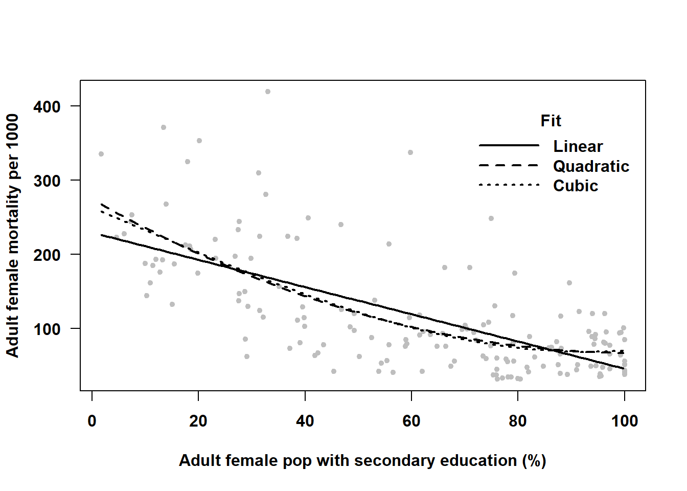
Figure 4.8: Using linear regression to fit a curve
In this example, Figure 4.8 confirms our conclusions from the statistical tests – the quadratic curve fits the data better than a straight line, and the cubic is not an improvement over the quadratic. So what is the relationship between nations’ adult female mortality rate and secondary school attainment? Based on this data, it appears that the mortality rate is lower in nations with greater secondary school attainment, but only for those with low to moderate attainment. Among those with the highest attainment, there is no relationship (the curve levels off at the higher values of \(X\)). A linear fit underestimates the slope among countries with lower attainment and overestimates the slope among those with higher attainment.
Overall test of a predictor modeled as a polynomial
What if we want a single overall test for a predictor that is fit using a polynomial? For a linear predictor, this was easy – we simply read the p-value from the regression output. But when you have a polynomial of order two (quadratic) or greater, the predictor is modeled using more than one term. As when we tested a categorical variable with more than two levels, we need an overall multiple df test of all the terms at the same time. In general, we need to compare the model that includes \(X\) as a polynomial to a reduced model that excludes \(X\) altogether. The anova() (lowercase a) function can accomplish this goal.
What went wrong? fit.poly.2 included the outcome mort_adult_f as well as the predictor educ_f whereas fit.reduced only included mort_adult_f. There were missing values in educ_f that resulted in the available observations being different for the two fits. Comparing the sample sizes used in each regression verifies that they are not the same.
## [1] 162## [1] 181How do we solve this? lm() has a subset option which can be used to remove cases with missing values for the variable that was used in fit.poly.2 but not fit.reduced. (Had we removed missing data before doing any of these analyses, this would not have been an issue.)
# Reduced model with correct sample
fit.reduced <- lm(mort_adult_f ~ 1, data = unhdd,
subset = complete.cases(educ_f))
# Compare reduced and full models
anova(fit.reduced, fit.poly.2)
## Analysis of Variance Table
##
## Model 1: mort_adult_f ~ 1
## Model 2: mort_adult_f ~ educ_f + I(educ_f^2)
## Res.Df RSS Df Sum of Sq F Pr(>F)
## 1 161 1028500
## 2 159 530058 2 498442 74.8 <0.0000000000000002 ***
## ---
## Signif. codes: 0 '***' 0.001 '**' 0.01 '*' 0.05 '.' 0.1 ' ' 1The “Df” column has a 2 because this is a 2 degree of freedom test; we are testing two terms simultaneously – the linear term educ_f and the quadratic term I(educ_f^2). According to the Analysis of Variance Table, we can reject the null hypothesis that both of these terms have coefficients equal to \(0\) and conclude that there is a significant association between secondary school attainment and mortality rate among adult females (p <.001). That is, the quadratic curve fits significantly better than a horizontal line at the mean outcome (no association). As before, be careful when using p-values to compare models. A visualization such as Figure 4.8 is valuable for clarifying the magnitude of differences between competing models. In this case, the figure is consistent with the hypothesis test – the quadratic model is meaningfully different from a horizontal line.