5.18 Checking the constant variance assumption
Not only does the assumption \(\epsilon \sim N(0, \sigma^2)\) imply normality of errors, it also implies that the variance of the errors (\(\sigma^2\)) is the same for every observation. In particular, since observations have different predictor values, this implies that the variance does not depend on any of the predictors or on the fitted values (which are linear combinations of predictor values). This is the constant variance (or homoscedasticity) assumption. For example, in Figure 5.36, the SLR on the left meets the constant variance assumption, while the one on the right does not.
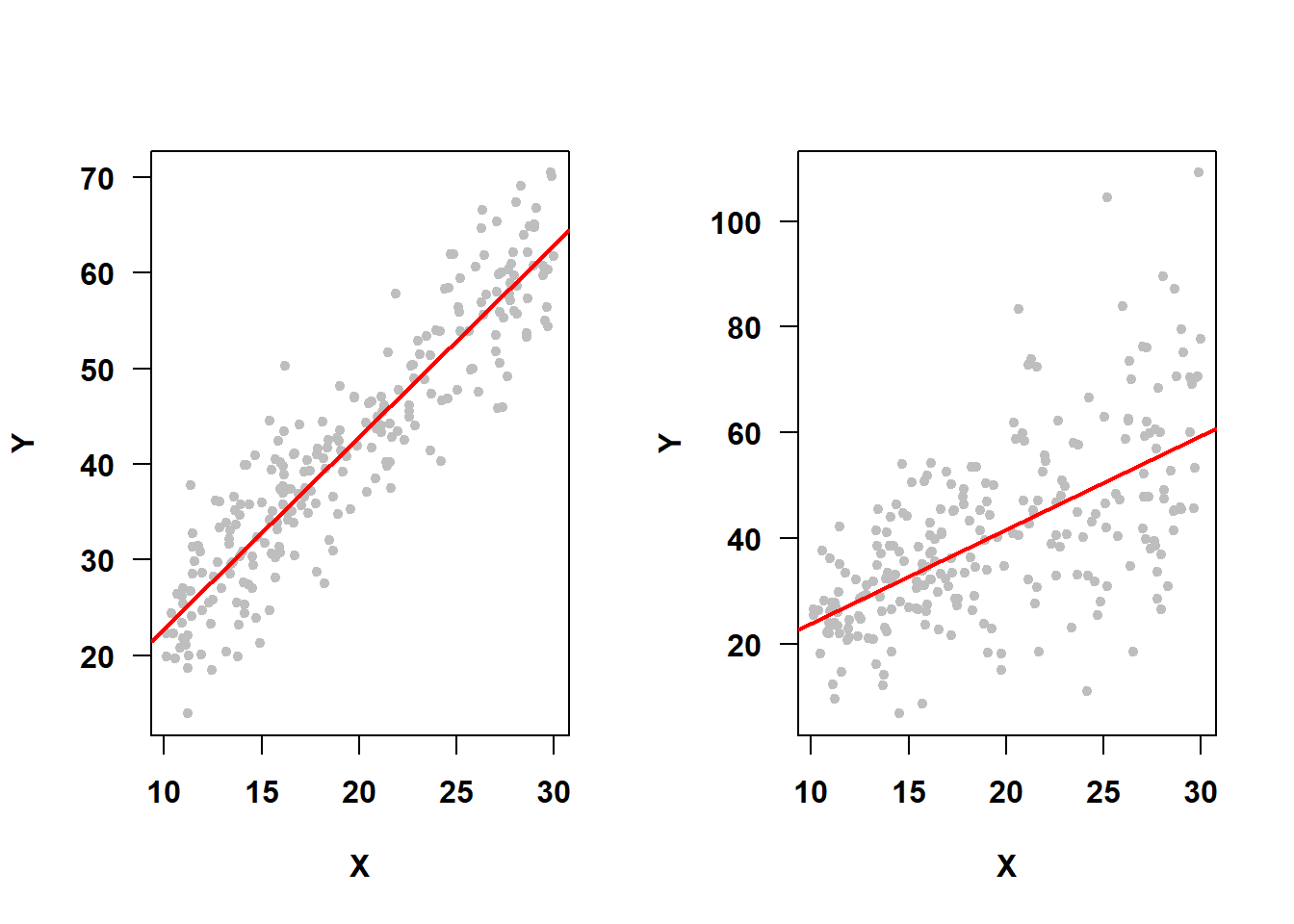
Figure 5.36: Constant variance assumption met vs. not met
5.18.1 Impact of non-constant variance
A violation of the constant variance assumption results in inaccurate confidence intervals and p-values, even in large samples, although regression coefficient estimates will still be unbiased (H. White 1980; Hayes and Cai 2007).
5.18.2 Diagnosis of non-constant variance
In SLR, the errors are assumed to have about the same amount of vertical variation from the regression line no matter where you are on the line, and this can be easily visualized, as in Figure 5.36, since there is just one predictor. In MLR, we visually diagnose the appropriateness of the constant variance assumption by examining a plot of residuals vs. fitted values (and, if we want to dig deeper, plots of residuals vs. each predictor) using car::residualPlots() (Fox, Weisberg, and Price 2024; Fox and Weisberg 2019). If the constant variance assumption is met, the spread of the points in the vertical direction should not vary much as you move in the horizontal direction.
Example 5.1 (continued): Evaluate the constant variance assumption for the MLR of fasting glucose on waist circumference, smoking status, age, gender, race, and income.
The residual vs. fitted value plot leads to the conclusion that we have non-constant variance since the variance is larger for larger fitted values (Figure 5.37).
# Residuals vs. fitted values
# fitted = T requests the residual vs. fitted plot
# terms = ~ 1 suppresses residual vs. predictor plots
# tests = F and quadratic = F suppresses hypothesis tests
# (see ?car::residualPlots for details)
car::residualPlots(fit.ex5.1,
                   pch=20, col="gray",
                   fitted = T, terms = ~ 1,
                   tests = F, quadratic = F)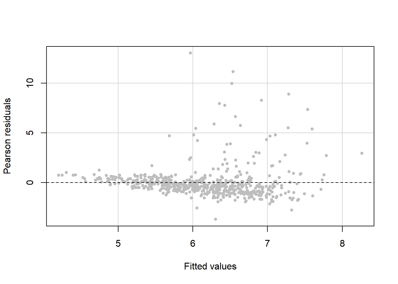
Figure 5.37: Residual vs. fitted plot to check the constant variance assumption
Examine residual vs. predictor plots for each predictor to see if the non-constant variance problem is related to any predictors more than others (Figure 5.38). In this example, these plots do not seem to add any information to the residual vs. fitted plot shown in Figure 5.37.
# Residuals vs. predictors
# fitted = F suppresses the residual vs. fitted plot
# ask = F prevents R from pausing and asking you to press
#     "Enter" to see additional plots
# layout = c(3,2) tells R to plot 6 panels per plot
#     in 3 rows and 2 columns
car::residualPlots(fit.ex5.1,
                   pch=20, col="gray",
                   fitted = F,
                   ask = F, layout = c(3,2),
                   tests = F, quadratic = F)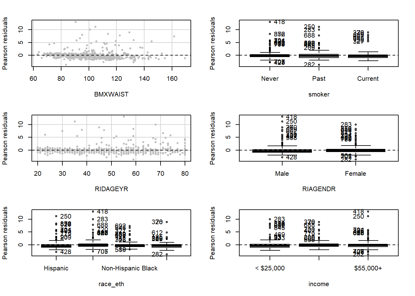
Figure 5.38: Residual vs. predictor plots to check the constant variance assumption
You can get all of these plots with one call to car::residualPlots() using the following syntax.
5.18.3 Potential solutions for non-constant variance
- Variance stabilizing transformation: A transformation of the outcome \(Y\) used to correct non-constant variance is called a “variance stabilizing transformation”. Again, common transformations are the natural logarithm, square root, inverse, and Box-Cox (Section 5.19).
- Advanced methods such as weighted or generalized least squares can be used to handle non-constant variance. These methods are beyond the scope of this text but see, for example, the
weightsoption in?lm(Foley 2019) and?nlme::gls(J. Pinheiro, Bates, and R Core Team 2025). - Non-constant variance may co-occur with non-linearity and/or non-normality. Again, check all the assumptions, resolve the most glaring assumption failure first, and then re-check all the assumptions.