5.21 Collinearity
An important step in the process of fitting an MLR is checking for collinearity between predictors. This step was not needed in SLR because there was only one predictor.
Here’s an extreme example which helps illustrate the concept. Suppose you want to know the relationship between fasting glucose and weight, and you fit a regression model that includes both weight in kilograms and weight in pounds. Clearly, these two predictors are redundant since they only differ in their units. With either one in the regression model, the other adds no new information. That is called perfect collinearity and it is mathematically impossible to include both in the model – you cannot estimate distinct regression coefficients for both predictors.
You also can have approximate collinearity. Suppose instead of weight in kilograms and weight in pounds, you have weight in kilograms and body mass index (BMI = weight/height2). While weight and BMI are not exactly redundant, they are highly related. In this case, it is mathematically possible to include both in the model, but their regression coefficients are difficult to estimate accurately (they will have large variances) and will be difficult to interpret. The regression coefficient for weight is the difference in mean outcome associated with a 1-unit difference in weight while holding BMI constant. But in order to vary weight while holding BMI constant you have to vary height, as well. The “effect of greater weight adjusted for BMI” is therefore actually the “effect of greater weight and greater height”, a combination of the effects of weight and height. In general, when two or more predictors are collinear, the interpretation of each while holding the other(s) fixed becomes more complicated.
Two predictors are perfectly collinear if their correlation is –1 or 1 (e.g., weight in kilograms and weight in pounds). The term “collinear” comes from the fact that one predictor (\(X_1\)) can be written as a linear combination of the other (\(X_2\)) as \(X_1 = a + b X_2\). If you were to plot the pairs of points \((x_{i1}, x_{i2})\) for all the cases, they would fall exactly on a line.
Examples of perfect collinearity include:
- Two predictors that are exactly the same \((X_1 = X_2)\);
- One predictor is twice the other \((X_1 = 2 X_2)\); and
- One predictor is 3 less than twice the other \((X_1 = -3 + 2 X_2)\).
If two predictors are perfectly collinear, then they are completely redundant for the purposes of linear regression. You could put either one in the model and the fit would be identical. Unless they are exactly the same (\(X_1 = X_2\)), you will get a different slope estimate using one or the other, but their p-values will be identical. If you put them both in the regression model at the same time, however, R will estimate a regression coefficient for just one of them, as shown in the following code.
# To illustrate...
# Generate random data from a standard normal distribution
set.seed(2937402)
y <- rnorm(100)
x <- rnorm(100)
# Create z perfectly collinear with x
z <- -3 + 2*x
lm(y ~ x + z)
##
## Call:
## lm(formula = y ~ x + z)
##
## Coefficients:
## (Intercept) x z
## -0.0776 0.1418 NAThe problem is actually worse, however, for approximate collinearity because, if you put both in the model, R will estimate a regression coefficient for each but will have trouble estimating their unique contributions and you could get strange results, such as one large negative and one large positive estimated \(\beta\) and large standard errors for the estimates (implying that even with only a slightly different sample of individuals you may get very different estimates of the \(\beta\)s).
Two predictors that are approximately collinear are essentially measuring the same thing and so should have about the same association with the outcome. But when each is adjusted for the other, the results for each can be quite unstable and quite different from each other. In the example below, the second predictor is identical to the first except for having some random noise added. Compare their unadjusted and adjusted associations with the outcome.
# Generate random data but make the collinearity approximate
set.seed(2937402)
y <- rnorm(100)
x <- rnorm(100)
# Create z approximately collinear with x
z <- x + rnorm(100, sd=0.05)
# Each predictor alone
round(summary(lm(y ~ x))$coef, 4)
## Estimate Std. Error t value Pr(>|t|)
## (Intercept) -0.0776 0.1020 -0.7601 0.4490
## x 0.1418 0.1087 1.3045 0.1951## Estimate Std. Error t value Pr(>|t|)
## (Intercept) -0.0783 0.1021 -0.767 0.4449
## z 0.1394 0.1079 1.292 0.1995## Estimate Std. Error t value Pr(>|t|)
## (Intercept) -0.0742 0.1034 -0.7176 0.4747
## x 0.7256 2.3995 0.3024 0.7630
## z -0.5799 2.3811 -0.2436 0.8081Each predictor individually has a regression slope of about 0.14 with a standard error of about 0.11. However, when attempting to adjust for each other, their slopes are now in opposite directions and their standard errors are around 2.4! Again, a large standard error means that if you happened to have drawn a slightly different sample, you might end up with very different regression coefficient estimates in the model with both x and z – the results are not stable. If you want to verify this, re-run the above code multiple times starting after set.seed() (so it is not reset to the same value each time), and compare the results.
Going back to our example of weight and BMI, we can see that in our NHANES fasting subsample dataset these two predictors are highly collinear (Figure 5.45). The points do not fall exactly on a line, but they are generally close. Thus, weight and BMI seem to be approximately collinear. This makes sense because BMI is a measure of body mass computed as weight normalized by stature.
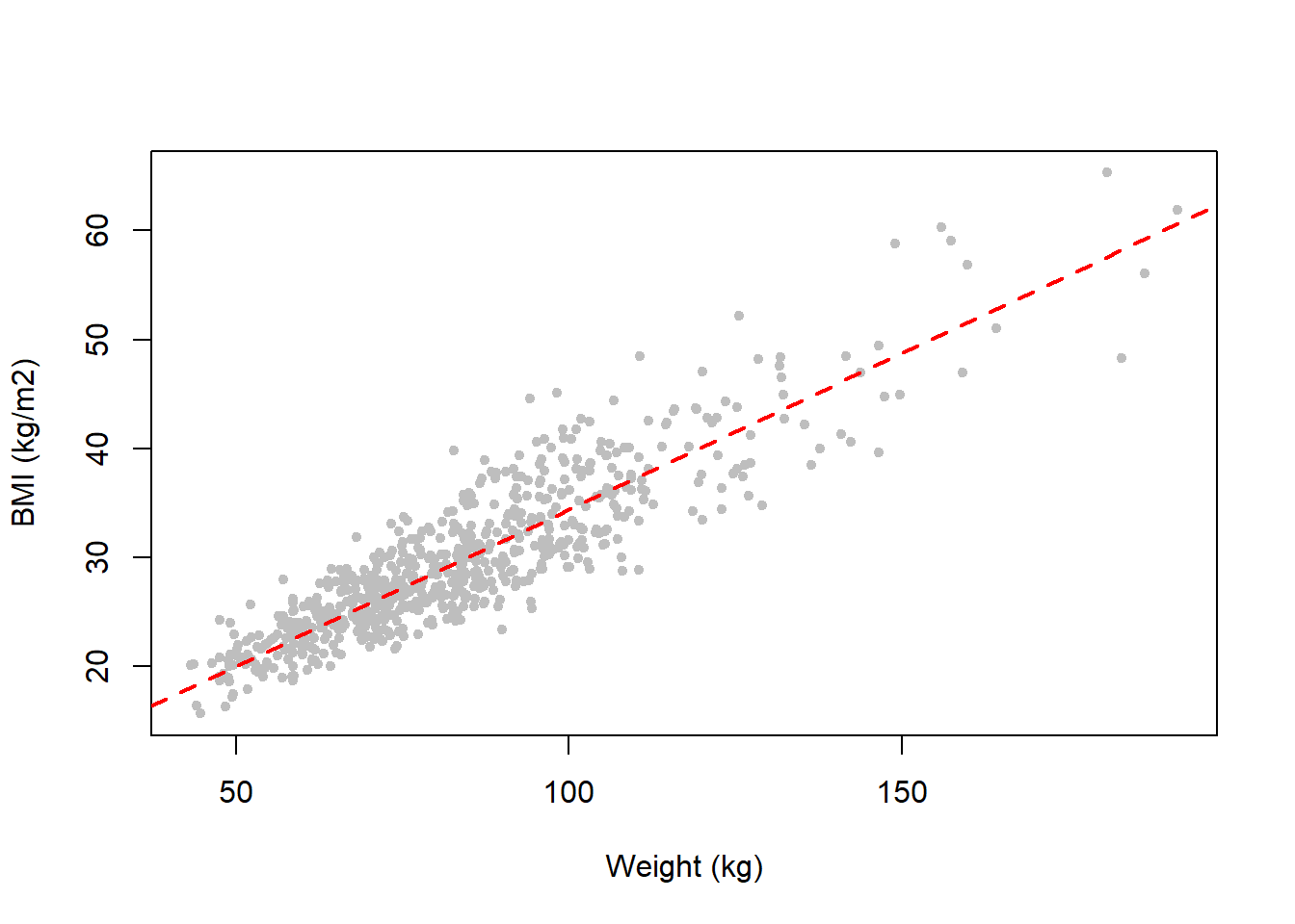
Figure 5.45: Body mass index and weight are highly collinear
All of the above examples were of pairwise collinearity. You can have collinearity between groups of predictors, as well, if some linear combination of one group of predictors is approximately equal to a linear combination of some other predictors. Such situations are harder to detect visually. However, in the following section, we will use a numeric diagnostic tool to help us detect collinearity even among groups of predictors.
5.21.1 Diagnosis of collinearity
The statistic we will use to diagnose collinearity is the variance inflation factor (VIF). For each predictor, the VIF measures how much the variance of the regression coefficient estimate is inflated due to correlation between that predictor and the others. Compute VIFs using the car::vif() function (Fox, Weisberg, and Price 2024; Fox and Weisberg 2019).
5.21.1.1 VIFs when all predictors are continuous
Example 5.6: Use VIFs to evaluate the extent of collinearity in the regression of the outcome systolic blood pressure (sbp) on the predictors age (RIDAGEYR), weight (BMXWT), BMI (BMXBMI), and height (BMXHT) using NHANES 2017-2018 examination data from adults (nhanes1718_adult_exam_sub_rmph.Rdata). First, fit the regression model. Second, call car::vif() with the regression fit as the argument.
load("Data/nhanes1718_adult_exam_sub_rmph.Rdata")
nhanes <- nhanes_adult_exam_sub # Shorter name
rm(nhanes_adult_exam_sub)

fit.ex5.6 <- lm(sbp ~ RIDAGEYR + BMXWT + BMXBMI + BMXHT, data = nhanes)
car::vif(fit.ex5.6)
## RIDAGEYR BMXWT BMXBMI BMXHT
## 1.014 88.835 69.934 18.764One of the VIFs is near 1, while the other three are much larger. How do we interpret the magnitude of VIFs? How large is “too large”? Unfortunately, there is no clear-cut answer to that question. We do know that a value of 1 is ideal – that indicates that the variance of that predictor’s regression coefficient estimate is not inflated at all by the presence of other predictors. Values above 2.5 may be of concern (Allison 2012), and values above 5 or 10 are indicative of a more serious problem. In this example height, weight, and BMI clearly have serious collinearity issues; their variances are being inflated 19- to 89-fold by their collective redundancy.
5.21.1.2 Generalized VIFs when at least one predictor is categorical
Recall that a categorical predictor with \(L\) levels will be entered into a model as \(L-1\) dummy variables (\(L-1\) vectors of 1s and 0s). Why \(L-1\)? Because if you included all \(L\) of them the vectors would sum up to a vector of all 1s (since every observation falls in exactly one category) and that would be perfect collinearity. So one is always left out (the reference level).
Example 5.6 examined collinearity among predictors that were all continuous. What happens if there are any categorical predictors? It turns out that the usual VIFs computed on a model with a categorical predictor will differ depending on which level is designated as the reference level. In addition to getting inconsistent results, we are not interested in the VIF for each individual level of a categorical predictor, but rather of the predictor as a single entity. Fortunately, car::vif() automatically gives us a consistent VIF, called the generalized VIF (GVIF) (Fox and Monette 1992), that is the same for each categorical predictor no matter the reference level, as long as the predictor is coded as a factor.
Example 5.7: Evaluate the extent of the collinearity in the regression of systolic blood pressure on the predictors age, BMI, height, and smoking status using our NHANES 2017-2018 examination subsample of data from adults (same dataset as in Example 5.6).
## GVIF Df GVIF^(1/(2*Df))
## RIDAGEYR 1.052 1 1.026
## BMXBMI 1.006 1 1.003
## BMXHT 1.051 1 1.025
## smoker 1.081 2 1.020The generalized VIF is found in the GVIF column. The GVIF^(1/(2*Df)) column is the adjusted generalized standard error inflation factor (aGSIF) and is equal to the square-root of GVIF for continuous predictors and categorical predictors with just two levels (since, for those, Df = 1). Fox and Monette (1992) recommend using the aGSIF, however, since for categorical predictors with more than two levels it adjusts for the number of levels allowing comparability with the other predictors. A consequence is that when using aGSIF, we must take the square-root of our rules of thumb for what is a large value – aGSIF values above \(\sqrt{2.5}\) (1.6) may be of concern, and values above \(\sqrt{5}\) or \(\sqrt{10}\) (2.2 or 3.2) are indicative of a more serious problem. Alternatively, you could square the aGSIF values and compare them to our original rule of thumb cutoffs.
Thus, the aGSIF for the three-level variable “smoker” is 1.02. In this example, the predictors do not exhibit strong collinearity (all the aGSIFs are near 1).
Run the code below if you would like to verify that the usual VIFs depend on which level is left out as the reference level but the GVIFs and aGSIFs remain unchanged.
# VIFs depend on the reference level
tmp <- nhanes %>%
mutate(smoker1 = as.numeric(smoker == "Never"),
smoker2 = as.numeric(smoker == "Past"),
smoker3 = as.numeric(smoker == "Current"))
fit_ref1 <- lm(sbp ~ RIDAGEYR + BMXBMI + BMXHT + smoker2 + smoker3, data = tmp)
fit_ref2 <- lm(sbp ~ RIDAGEYR + BMXBMI + BMXHT + smoker1 + smoker3, data = tmp)
fit_ref3 <- lm(sbp ~ RIDAGEYR + BMXBMI + BMXHT + smoker1 + smoker2, data = tmp)
car::vif(fit_ref1)
car::vif(fit_ref2)
car::vif(fit_ref3)
# GVIF and aGSIF do not depend on the reference level
car::vif(lm(sbp ~ RIDAGEYR + BMXBMI + BMXHT + smoker, data = nhanes))
tmp <- nhanes %>%
mutate(smoker = relevel(smoker, ref = "Past"))
car::vif(lm(sbp ~ RIDAGEYR + BMXBMI + BMXHT + smoker, data = tmp))
tmp <- nhanes %>%
mutate(smoker = relevel(smoker, ref = "Current"))
car::vif(lm(sbp ~ RIDAGEYR + BMXBMI + BMXHT + smoker, data = tmp))
# (results not shown)5.21.1.3 VIFs when there is an interaction or polynomial terms
Collinearity between terms involved in an interaction can be ignored (Allison 2012). This applies also to collinearity between terms that together define a polynomial curve (e.g., \(X\), \(X^2\), etc.). In general, centering continuous predictors will reduce the collinearity. However, the sort of collinearity that is removed by centering actually has no effect on the fit of the model, only on the interpretation of the intercept and the main effects of predictors involved in the interaction. If you have interactions in the model, or multiple terms defining a polynomial, compute the VIFs or aGSIFs using a model without the interactions or higher order polynomial terms. Alternatively, instead of entering a polynomial using individual terms, use the poly() function. For example, for a quadratic in BMXWT, instead of entering BMXWT + I(BMWXT^2), enter poly(BMXWT, 2) into lm(). car::vif() will then return one aGSIF value for the entire polynomial; note however, that the way polynomials are parameterized with poly() is different than in our examples where we entered terms individually.
5.21.1.4 VIF summary
- If all predictors in a model are continuous and/or binary (two levels) then
car::vif()returns VIFs and our rule of thumb for what is large is that values above 2.5 may be of concern and values above 5 or 10 are indicative of a more serious problem. - If any predictors in a model are categorical with more than two levels then
car::vif()returns both GVIF and aGSIF values. Use the aGSIF values to evaluate collinearity since that allows predictors with differentDf(different number of terms in the model) to be comparable. For aGSIFs, our rule of thumb for what is large is that values above 1.6 may be of concern and values above 2.2 or 3.2 are indicative of a more serious problem. - Our rule of thumb regarding what is a large amount of inflation is arbitrary. It is useful as a guide, but there is no requirement to apply it strictly.
- If you have interactions in the model, or multiple terms defining a polynomial, compute the VIFs or aGSIFs using a model without the interactions or higher order polynomial terms. Alternatively, for polynomials, use
poly()when fitting the model.
5.21.2 Impact of collinearity
When there is perfect collinearity, R will drop out predictors until that is no longer the case and so there is no impact on the final regression results. When there is approximate collinearity, however, there may be inflated standard errors and difficulty interpreting coefficients.
Example 5.7 (continued): It is reasonable to guess that the main driver of the collinearity is the strong correlation between weight and BMI. Compare the regression coefficients, their standard errors, and their p-values with and without weight in the model. First, create a complete-case dataset so differences between the models are not due to having different observations.
# Create a complete-case dataset so both models use the same sample
sbpdat <- nhanes %>%
select(sbp, RIDAGEYR, BMXWT, BMXBMI, BMXHT) %>%
drop_na()
# With weight in the model
fit_wt <- lm(sbp ~ RIDAGEYR + BMXWT + BMXBMI + BMXHT, data = sbpdat)
# After dropping weight due to high collinearity
fit_nowt <- lm(sbp ~ RIDAGEYR + BMXBMI + BMXHT, data = sbpdat)| Term | B | SE | p | VIF | B | SE | P | VIF |
|---|---|---|---|---|---|---|---|---|
| Intercept | 137.34 | 36.41 | <.001 | 73.52 | 8.96 | <.001 | ||
| Age | 0.4327 | 0.0292 | <.001 | 1.01 | 0.4348 | 0.0292 | <.001 | 1.01 |
| Weight | 0.3707 | 0.2050 | .071 | 88.8 | – | – | – | |
| BMI | -0.5093 | 0.5782 | .379 | 69.9 | 0.5287 | 0.0692 | <.001 | 1.00 |
| Height | -0.3029 | 0.2169 | .163 | 18.8 | 0.0787 | 0.0505 | .119 | 1.01 |
Table 5.4 shows how the results differ after removing weight from the model. As expected, since its VIF was near 1, the “Age” row does not change much. Note in particular that, up to four decimal places, its standard error (SE) is exactly the same. This is what it means for a VIF to be 1 – that the variance (the square of the SE) is inflated by a factor of 1, in other words not inflated at all, by the presence of the other predictors.
Compare this, however, to the rows for “BMI” and “Height”. After removing weight from the model, their estimates change drastically; both change direction, going from negative to positive. Also, their standard errors decrease dramatically, indicating that they are more precisely estimated. The squares of the ratios of their SEs with and without weight in the model are approximately the same as their VIFs in the model that includes weight.
## [1] 69.74## [1] 18.49The reason the variances decrease so much is that the definitions of “BMI holding other predictors fixed” and “height holding other predictors fixed” change after removing weight, with the old quantities (effects of BMI and height when holding age and weight constant) being much harder to estimate accurately (and harder to interpret) than the new (effects of BMI and height when holding age constant). Also, whereas “BMI when holding age, weight, and height constant” was not statistically significant (p = .379), “BMI when holding age and height constant” is (p <.001). Finally, after removing weight from the model, the VIFs for the remaining predictors are all near 1.
5.21.3 Potential solutions for collinearity
There are multiple ways to deal with collinearity:
- Remove one or more predictors from the model, or
- Combine predictors (e.g., average, sum, difference).
One could also try a biased regression technique such as LASSO or ridge regression. Those methods are beyond the scope of this text but see, for example, the R package glmnet (Friedman, Hastie, and Tibshirani 2010)).
5.21.3.1 Remove predictors to reduce collinearity
Ultimately, you want a set of predictors that are not redundant. One solution is to remove predictors suspected of being problematic, one at a time, and see if the VIFs become smaller.
Before removing any predictors, check the extent of missing data in the dataset. On one hand, when comparing VIFs between models with different predictors, each model should be fit to the same set of observations, which means starting with a complete case dataset. On the other hand, one or more predictors might have a much larger number of missing values than the others. In that case, it might be best to remove the predictors with a lot of missing values first, create a complete case dataset based on the remaining predictors, and then compare VIFs between models with different predictors.
Example 5.7 (continued): Remove one predictor at a time and see how the VIFs change. Use the complete case dataset created above so any differences are due to removing predictors rather than differing sets of observations with non-missing values.
## RIDAGEYR    BMXWT   BMXBMI    BMXHT
## 1.014 88.835 69.934 18.764## RIDAGEYR BMXBMI BMXHT
## 1.012 1.000 1.013## RIDAGEYR BMXWT BMXHT
## 1.012 1.271 1.284## RIDAGEYR BMXWT BMXBMI
## 1.010 4.794 4.786With all four predictors in the model, BMI, weight, and height each exhibit high collinearity. After removing them one at a time we see that, in fact, weight and BMI are the problem variables (the VIFs are only large when both remain in the model). In this example, removing weight from the model best resolved the collinearity issue (the VIFs are smallest when weight was removed). In other examples, you may have to remove more than one predictor to obtain VIFs that are all small.
5.21.3.2 Combine predictors to reduce collinearity
Simply removing predictors is often the best solution. At other times, you really would like to keep all the predictors. In that case, combining them in some way may work. Common methods of combining predictors include taking the average, the sum, or the difference.
Example 5.8: Using the Natality dataset (see Appendix A.3), examine the extent of collinearity in the regression of the outcome birthweight (DBWT, g) on the ages of the mother (MAGER) and father (FAGECOMB) and resolve by combining predictors.
load("Data/natality2018_rmph.Rdata")
fit.ex5.8 <- lm(DBWT ~ MAGER + FAGECOMB, data = natality)
round(summary(fit.ex5.8)$coef, 4)
## Estimate Std. Error t value Pr(>|t|)
## (Intercept) 3168.469 75.620 41.8999 0.0000
## MAGER 5.769 3.767 1.5317 0.1258
## FAGECOMB -2.519 3.067 -0.8215 0.4115## MAGER FAGECOMB
## 2.32 2.32Ignoring statistical significance, this model implies that (1) for a given father’s age, older mothers have children with greater birthweight and (2) for a given mother’s age, older fathers have children with lower birthweight. In this particular dataset, the two predictors are not highly collinear, but their VIFs are close to the rule of thumb cutoff of 2.5. We will attempt to reduce their collinearity by combining them to form two predictors that are less collinear.
Replacing a pair of correlated predictors \(X_1\) and \(X_2\) with their average \(Z_1 = (X_1 + X_2)/2\) and difference \(Z_2 = X_1 - X_2\) may result in a pair of less correlated predictors. In this example, the transformed predictors would be interpreted as “average parental age” and “parental age difference”.
natality <- natality %>%
  mutate(avg_parent_age        = (FAGECOMB + MAGER)/2,
         parent_age_difference =  FAGECOMB - MAGER)

fit.ex5.8_2 <- lm(DBWT ~ avg_parent_age + parent_age_difference, data = natality)
round(summary(fit.ex5.8_2)$coef, 4)
## Estimate Std. Error t value Pr(>|t|)
## (Intercept) 3168.469 75.620 41.900 0.0000
## avg_parent_age 3.250 2.483 1.309 0.1908
## parent_age_difference -4.144 3.202 -1.294 0.1958## avg_parent_age parent_age_difference
## 1.099 1.099Ignoring statistical significance, these results imply that (1) for a given age difference, older parents have children with greater birthweight and (2) for a given average parental age, parents with a larger age difference have children with lower birthweight. By combining the predictors, we have reduced collinearity while retaining the ability to draw conclusions based on the combination of ages of both parents.
In other cases, you might combine the collinear predictors into a single predictor by replacing them with their sum or average. For example, if you have a set of items in a questionnaire that all are asking about the same underlying construct, each on a scale from, say, 1 to 5 (e.g., Likert-scale items), you may be able to average them together to produce a single summary variable. If taking this approach, be sure all the items are on the same scale and if they are not then standardize them before summing or averaging. Also, make sure the ordering of responses has the same meaning – sometimes one item is asking about agreement with the underlying construct and another is asking about disagreement, resulting in a low score on one item having the same meaning as a high score on another. If you have items with different response orderings, change some of them until all are in the same direction. For example, you could reverse the ordering of items asking about disagreement (e.g., replace a 1 to 5 scale with scores of 5 to 1) so they match items asking about agreement. While summing or averaging variables may work to reduce collinearity, it is important to also assess whether such a sum is valid using methods such as Cronbach’s alpha and factor analysis (beyond the scope of this text but see, for example, ?psy::cronbach (Falissard 2022) and ?factanal).
In general, take time to think about how your candidate predictors are related to each other and to the outcome. Are some completely or partially redundant (measuring the same underlying concept)? That will show up in the check for collinearity. Remove or combine predictors in a way that aligns with your analysis goals.