5.17 Checking the linearity assumption
A linear regression model assumes that the average outcome is linearly related to each term in the model when holding all others fixed. That is why plotted unadjusted (Section 5.5) or adjusted (Section 5.8) linear regression lines are straight lines – the model assumes straight lines. However, the underlying population relationship might not be linear – in that case, a straight line may not be a good fit to the data. For example, in Figure 5.26, the SLR on the left meets the linearity assumption, while the one on the right (from Example 4.3) does not (the dashed line is a smoother added to illustrate the shape of the trajectory when relaxing the linearity assumption).
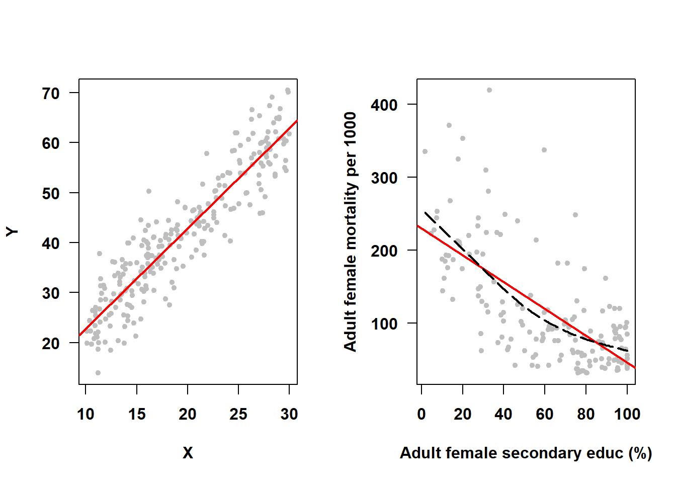
Figure 5.26: Linearity assumption met vs. not met
There is an aspect of the linearity assumption that must be clarified before proceeding. The assumption is linearity in “each term in the model”, not linearity in “each predictor”. Why this distinction? Because sometimes a predictor is expressed in the model using multiple terms. Recall that for Example 5.1, the MLR model is the following.
\[\begin{array}{rcl} \textrm{FG} & = & \beta_0 \\ & + & \beta_1 \textrm{WC} \\ & + & \beta_2 I(\textrm{Smoker = Past}) + \beta_3 I(\textrm{Smoker = Current}) \\ & + & \beta_4 \textrm{Age} \\ & + & \beta_5 I(\textrm{Gender = Female}) \\ & + & \beta_6 I(\textrm{Race = Non-Hispanic White}) + \beta_7 I(\textrm{Race = Non-Hispanic Black}) \\ & + & \beta_8 I(\textrm{Race = Non-Hispanic Other}) \\ & + & \beta_9 I(\textrm{Income = \$25,000 to <\$55,000}) + \beta_{10} I(\textrm{Income = \$55,000+}) + \epsilon \end{array}\]
For a continuous predictor (e.g., WC), the “term in the model” is the predictor itself. For a binary categorical predictor (e.g., gender), the “term in the model” is a single indicator function for one of the levels. In each of these cases, if you were to plot the mean outcome (holding all except this predictor fixed) vs. the predictor, you would see a straight line. For a continuous predictor, this is because the model assumes the relationship is linear, but in fact that assumption may be wrong and needs to be checked. For a binary predictor, the linearity assumption is always true – there are two means (the mean outcome at each level of the predictor) and a straight line always perfectly fits two points.
What about a categorical predictor with more than two levels (e.g., smoking status)? Figure 5.27 illustrates the unadjusted association between smoking status and fasting glucose in Example 5.1.
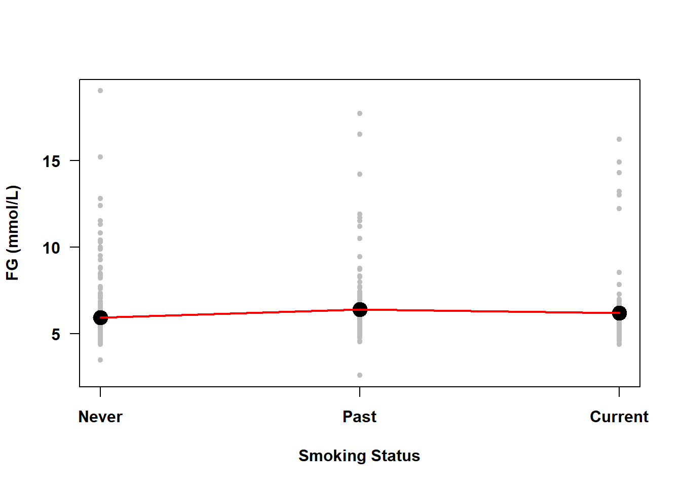
Figure 5.27: Categorical predictors do not violate the linearity assumption even if the plot appears non-linear
The line connecting the means at each level of smoking status is not straight. This is not, however, a violation of the linearity assumption as the “line” here was added after the fact just to connect the dots to provide a visual aid to discerning if any means are larger or smaller than the others – the line was not estimated by the regression model. If you were to plot the mean outcome vs. each individual indicator function, however, you would see just two means and, as mentioned above, a line always perfectly fits two points (Figure 5.28). Thus, even with categorical predictors with more than two levels, the underlying numeric indicator functions are each always linearly related to the outcome.
par(mfrow=c(1,2))
tmpdat <- nhanesf.complete %>%
  # Create an indicator function for each non-reference level
  mutate(Past    = factor(smoker == "Past"),
         Current = factor(smoker == "Current"))
plotyx("LBDGLUSI", "Past",    tmpdat,
       ylab = "FG (mmol/L)",
       xlab = "Smoking = Past")
plotyx("LBDGLUSI", "Current", tmpdat,
       ylab = "FG (mmol/L)",
       xlab = "Smoking = Current")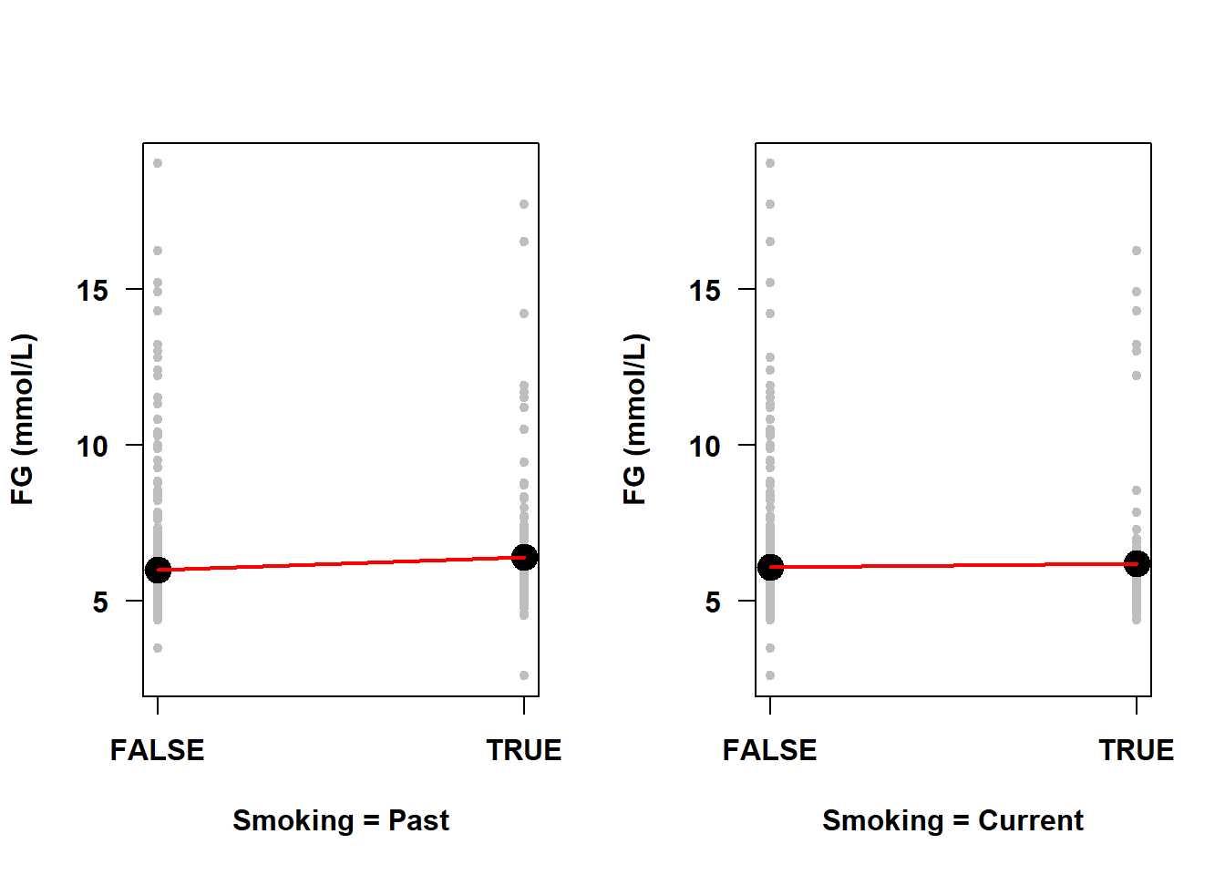
Figure 5.28: Linearity assumption met by default for indicator variables
Additionally, there are many applications of linear regression where you can fit something other than a straight line, as we did in Section 4.8 when we fit a polynomial, or if we transform variables in some other way (e.g., a log-transformation of the outcome or a predictor). Technically, the “linear” in “linear regression” refers to the outcome being linear in the parameters, the \(\beta\)s. The mathematics behind fitting a regression line involves taking the derivative of \(Y\) with respect to the parameters and when the relationship is linear the resulting equations can be solved. When the relationship is non-linear, however, estimating the parameters of the model requires more complex algorithms.
When we used a polynomial curve for a single predictor, we still could use “linear” regression because we could express the polynomial function as the sum of functions. You can use linear regression to fit any non-linear function of a predictor \(X\) that can be expressed as a sum of the product of coefficients and functions of \(X\) that do not have any coefficients inside the function. For example,
\[\begin{array}{lrcl} \text{1. Linear regression (quadratic polynomial):} & Y & = & \beta_0 + \beta_1 X + \beta_2 X^2 + \epsilon \\ \text{2. Linear regression (log-transformed predictor):} & Y & = & \beta_0 + \beta_1 \log(X) + \epsilon \\ \text{3. Linear regression (log-transformed outcome):} & \log(Y) & = & \beta_0 + \beta_1 X + \epsilon \\ \text{4. Non-linear regression:} & Y & = & \beta_0 + \frac{\beta_1 X}{\beta_2 + \beta_3 (X+1)} + \epsilon \\ \text{5. Non-linear regression:} & Y & = & \beta_0 e^{\beta_1 X} \epsilon \end{array}\]
In the first three examples above, even though the \(Y\) vs. \(X\) relationship is non-linear, the (possibly transformed) outcome is linearly related to each term in the model. That is not the case with the final two examples, which are non-linear regression models. Sometimes, however, you can convert a non-linear regression model into a linear one, but not always. To fit the fourth model above, you would have to use non-linear regression. But for the fifth, a natural log transformation of \(Y\) converts the model into the linear model \(Y^* = \beta_0^* + \beta_1 X + \epsilon^*\) where \(Y^* = \log(Y)\), \(\beta_0^* = \log(\beta_0)\) and \(\epsilon^* = \log(\epsilon)\).
In summary:
- You only need to check the linearity assumption for continuous predictors. For a categorical predictor, the linearity assumption is always met for each of the indicator functions since a straight line always fits two points exactly.
- The MLR model assumes linearity between the (possibly transformed) outcome and each “term in the model”, each of which is either a (possibly transformed) continuous predictor or an indicator function for a level of a categorical predictor.
- In some cases, a transformation can convert a non-linear regression model into a linear regression model.
5.17.1 Impact of non-linearity
If the true model is not linear, then predictions based on a model that assumes linearity will be biased. For example, in the analysis of nation-level adult female mortality rate in Example 4.3 in Section 4.8, we found that if you predict mortality rate based on the linear fit, your prediction will be very different from the prediction based on the better fitting non-linear relationship, as shown in Figure 5.29 At some predictor values, the linear fit would result in an overestimate of the mean outcome, at others an underestimate.
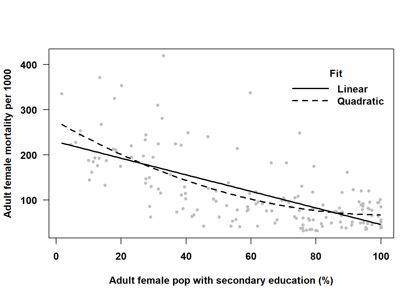
Figure 5.29: Not accounting for non-linearity can lead to biased predictions
Also, importantly, the test of significance of the regression coefficient for the predictor is testing the significance of a linear relationship. But if the true form of the relationship is not linear, then this is not the test you want.
5.17.2 Diagnosis of non-linearity
The linearity assumption requires that the \(Y\) vs. \(X\) relationship be linear when holding all other predictors fixed. A residual plot that takes that into account and is effective at diagnosing non-linearity is the component-plus-residual plot (CR plot), also known as a partial-residual plot. Create a CR plot for each continuous predictor using the car::crPlots() function (Fox, Weisberg, and Price 2024; Fox and Weisberg 2019).
Example 5.1 (continued): Check the linearity assumption using a CR plot for each continuous predictor (waist circumference, age). The plots are shown in Figure 5.30.
NOTE: The terms argument is used below to avoid outputting unnecessary diagnostic plots for categorical predictors. If all predictors in the model are continuous, you can omit the terms argument below and you will get a plot for each.
# Use the "terms" option to specify the continuous predictors
# Override the default smoother -- gamLine seems to work better
car::crPlots(fit.ex5.1, terms = ~ BMXWAIST + RIDAGEYR,
             pch=20, col="gray",
             smooth = list(smoother=car::gamLine))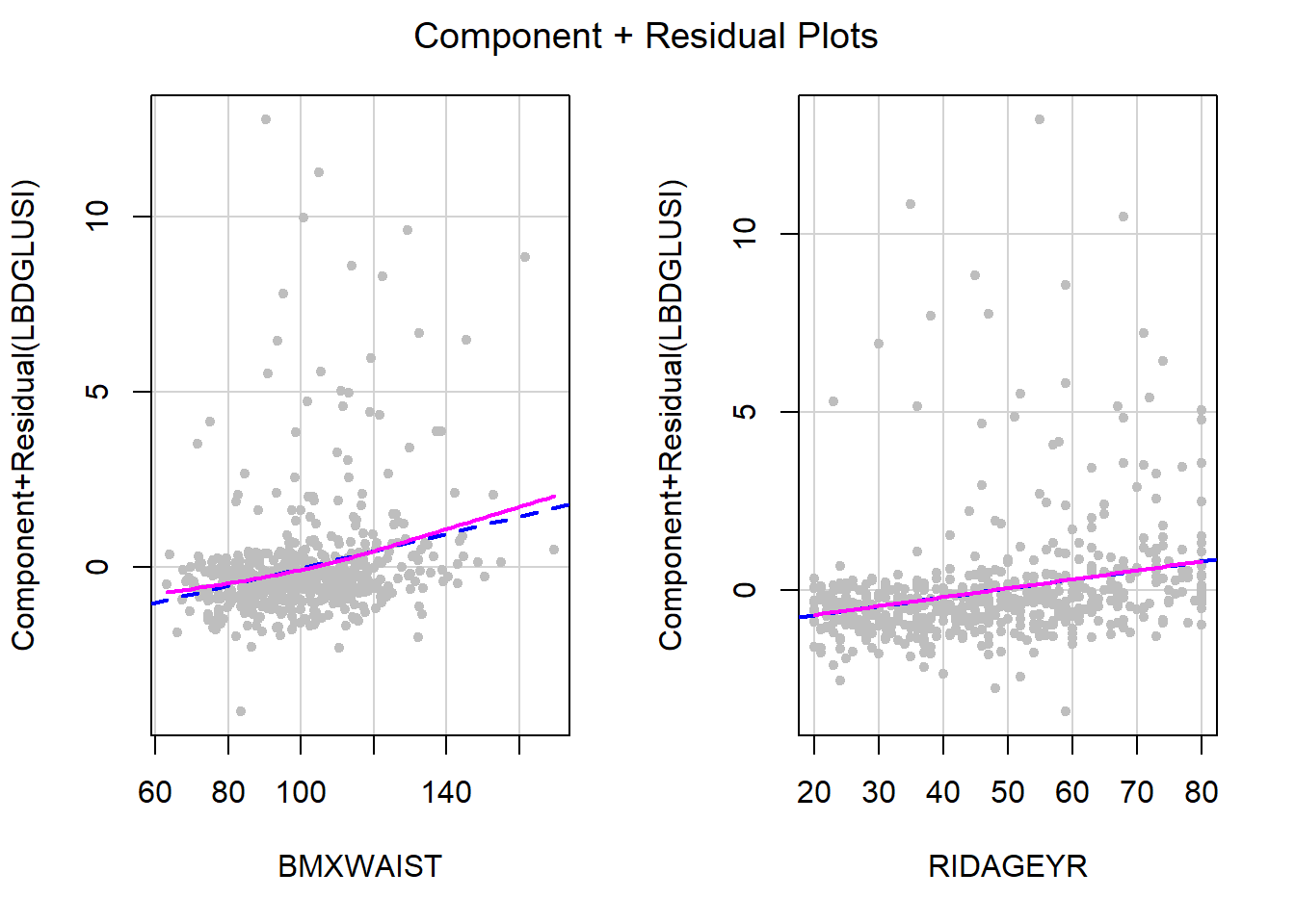
Figure 5.30: Residuals vs. predictors to check linearity assumption
In each panel, the raw predictor values are plotted on the horizontal axis. The vertical axis plots the residuals plus the specific contribution of \(X\), adjusted for all the other predictors in the model, \((\hat{\beta_j} x_{ij})\) added back in (the component). The dashed line is the linear regression of the component + residual vs. \(X\). If there were no linear association between \(Y\) and \(X\) after adjusting for all other predictors in the model, the dashed line would be a horizontal line at 0. The solid line is a smoother that relaxes the linearity assumption. In each panel, if the solid line falls exactly on top of the dashed line, then the linearity assumption is perfectly met for that predictor. In this example, age is linear, but there seems to be a slight non-linearity for waist circumference.
5.17.2.1 Checking linearity in a model with an interaction
If the model includes an interaction, the linearity assumption becomes more complicated to check (and car::crPlots() will return an error). Although not ideal, an approximate solution is to diagnose linearity in the model without any interactions. Another option is to stratify the data by one of the predictors in the interaction, run lm() separately at each level of that predictor, and check the linearity assumption in each of those models (none of which have an interaction anymore) using car::crPlots(). If the stratifying predictor is continuous, then you can approximate this method by creating a categorical version of that predictor first (see, for example, ?cut).
5.17.3 Potential solutions for non-linearity
- Fit a polynomial curve (see Section 4.8 and the example below).
- Transform \(X\) and/or \(Y\) to obtain a linear relationship. Common transformations are the natural logarithm, square root, and inverse. A Box-Cox transformation of the outcome may help, as well (Section 5.19). These transformations all assume \(X\) varies monotonically with \(Y\) (either \(X\) always increases with \(Y\) or always decreases with \(Y\)). A polynomial curve, however, can handle non-monotonic non-linearities (a curve that changes directions vertically).
- Use a spline function to fit a smoother (not discussed here, but see Harrell (2015) for more information).
- Transform \(X\) into a categorical variable (e.g., using tertiles or quartiles of \(X\) as cutoffs). It is generally better to not categorize a continuous predictor as you lose information and the cutoffs are arbitrary, but this method can be useful just to see what the trend looks like.
- Non-linearity may co-occur with non-normality and/or non-constant variance. As mentioned previously, check all the assumptions, resolve the most glaring assumption failure first, and then re-check all the assumptions.
Example 5.1 (continued): Above, we found that waist circumference violates the linearity assumption. Try adding a quadratic term and see if that helps.
fit.ex5.1.quad <- lm(LBDGLUSI ~ BMXWAIST + smoker + RIDAGEYR +
                       RIAGENDR + race_eth + income +
                       I(BMXWAIST^2), data = nhanesf.complete)
round(summary(fit.ex5.1.quad)$coef, 4)
## Estimate Std. Error t value Pr(>|t|)
## (Intercept) 5.7468 1.4313 4.0152 0.0001
## BMXWAIST -0.0301 0.0274 -1.1004 0.2715
## smokerPast 0.2089 0.1249 1.6720 0.0949
## smokerCurrent 0.0730 0.1509 0.4835 0.6288
## RIDAGEYR 0.0266 0.0034 7.8477 0.0000
## RIAGENDRFemale -0.3491 0.1055 -3.3098 0.0010
## race_ethNon-Hispanic White -0.5407 0.1459 -3.7069 0.0002
## race_ethNon-Hispanic Black -0.2770 0.1994 -1.3895 0.1650
## race_ethNon-Hispanic Other -0.0125 0.2163 -0.0576 0.9541
## income$25,000 to <$55,000 -0.0818 0.1627 -0.5026 0.6154
## income$55,000+ -0.0831 0.1471 -0.5650 0.5722
## I(BMXWAIST^2) 0.0003 0.0001 2.0085 0.0449The quadratic term is statistically significant; however, with a large sample size that might happen even if it does not change the model fit very much. Does it visually solve the failure of the linearity assumption? Enter each of the BMXWAIST terms, as well RIDAGEYR, into car::crPlots() and check the assumption again (Figure 5.31).
car::crPlots(fit.ex5.1.quad, terms = ~ BMXWAIST + I(BMXWAIST^2) + RIDAGEYR,
             pch=20, col="gray",
             smooth = list(smoother=car::gamLine))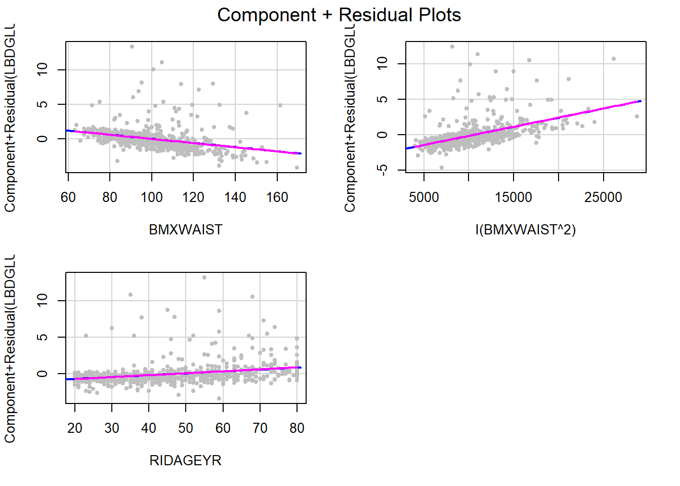
Figure 5.31: CR plots after adding a quadratic term
The linearity assumption is very well met now. It may seem strange that we have “linearity” when we have included waist circumference as a quadratic in the model! But remember that the linearity assumption has to do with each term in the model on its own, not with the entire quadratic polynomial for waist circumference. So as long as the CR plot shows linearity in each term individually, the linearity assumption is met.
5.17.4 Examples of non-linearities that are resolved by a transformation of the predictor
When the \(X\) values are highly skewed with a large range, which often happens with lab measurements or variables such as income or population size, then a log transformation often works well (Weisberg 1985).
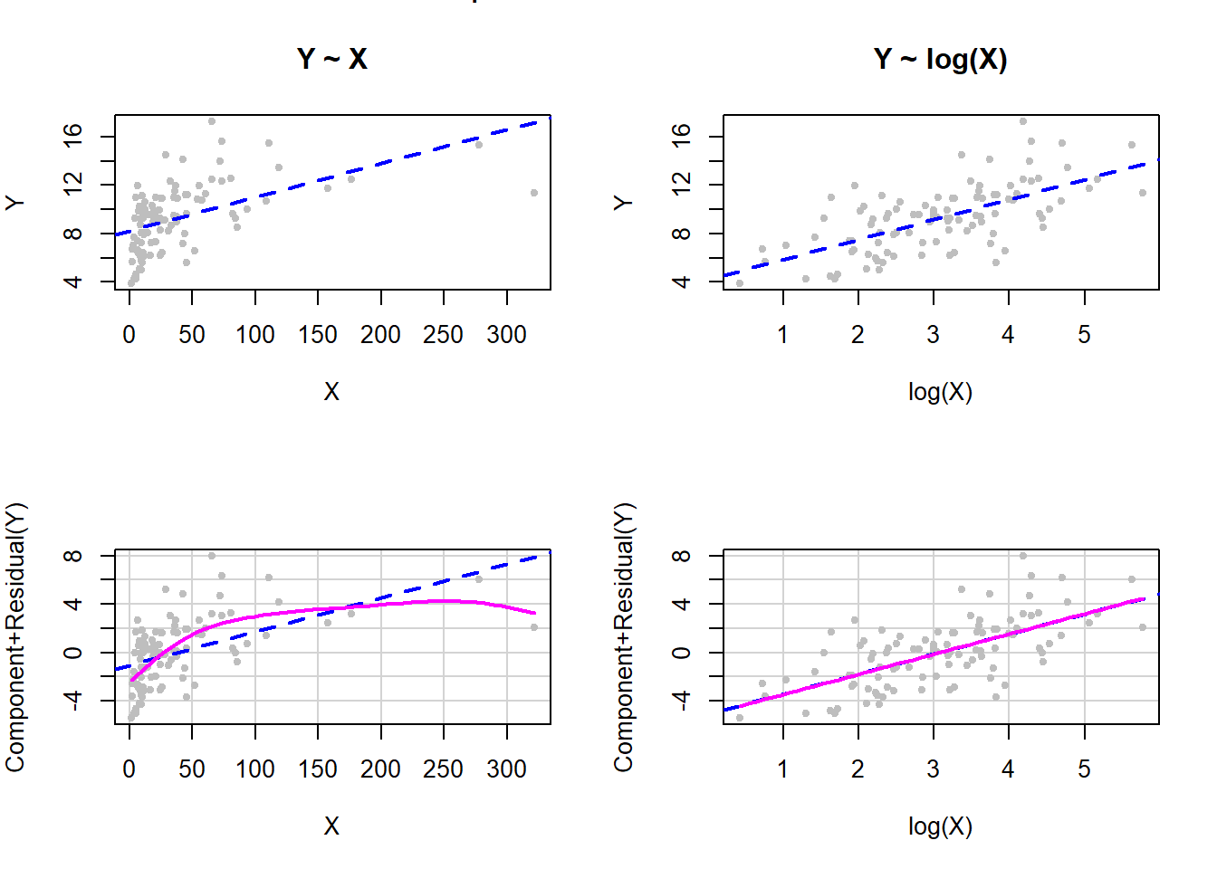
Figure 5.32: Log transformation of X to fix non-linearity
The top row of panels in Figure 5.32 are scatterplots of the outcome vs. the predictor, before (left panel) and after (right panel) the transformation. The panels on the bottom row are the corresponding CR plots. In this simulated example, the log transformation perfectly took care of the non-linearity. This illustrates the sort of \(Y\) vs. \(X\) relationship where a log transformation may help.
When the \(X\) values are skewed with a moderate range a square-root transformation often works well, as illustrated in Figure 5.33.
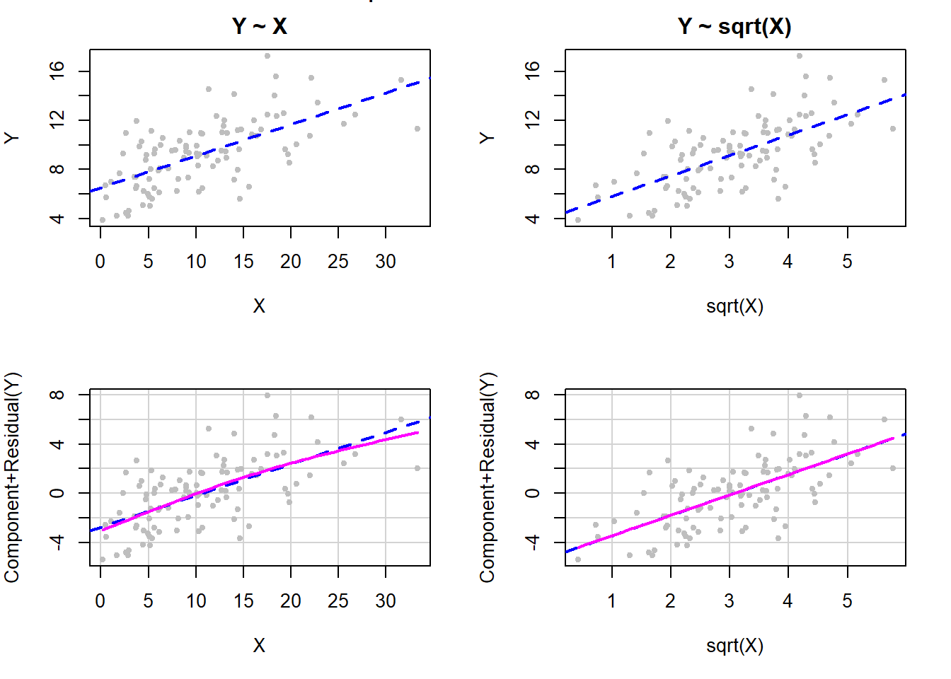
Figure 5.33: Square root transformation of X to fix non-linearity
When there are many \(X\) values near zero but with some larger values, as well, then an inverse transformation often works well (Weisberg 1985), as illustrated in Figure 5.34 (note that we multiply by –1 to preserve the ordering of the original variable).
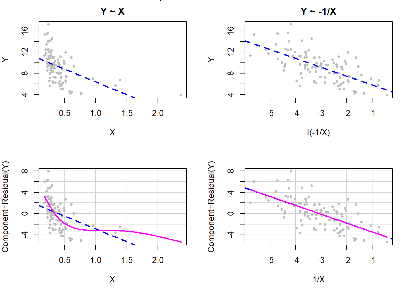
Figure 5.34: Inverse transformation of X to fix non-linearity
5.17.5 Changing the amount of smoothing in a CR plot
The default options allow the smoother in car::crPlots() to choose the amount of smoothing. Sometimes the smoother is too unstable and we would like to change the amount of smoothing. The k argument (demonstrated below) has a default value of –1, which results in automatic smoothing (what you get if you leave out the k option altogether as we did in the previous examples). If not the default, k must be at least 3 and larger values of k result in less smoothing.
Example 5.5: Use data from the United Nations 2020 Human Development Data (unhdd2020.rmph.rData, see Appendix A.2) (United Nations Development Programme 2020) and regress the outcome Human Development Index (hdi) on the predictor tuberculosis incidence (2018, per 100,000 people) (tb), after using a square root transformation, and check the linearity assumption with smoothing argument values of –1 (automatic smoothing), 3 (maximum smoothing that is not a line), 5, and 10 (Figure 5.35).
load("Data/unhdd2020.rmph.rData")
fit.ex5.5 <- lm(hdi ~ sqrt(tb), data = unhdd)

par(mfrow=c(2,2))
car::crPlots(fit.ex5.5, terms = ~ sqrt(tb),
             pch=20, col="gray",
             smooth = list(smoother=car::gamLine, k = -1))
title("Default (automatic) smoothing")
car::crPlots(fit.ex5.5, terms = ~ sqrt(tb),
             pch=20, col="gray",
             smooth = list(smoother=car::gamLine, k = 3))
title("k = 3 (maximum smoothing)")
car::crPlots(fit.ex5.5, terms = ~ sqrt(tb),
             pch=20, col="gray",
             smooth = list(smoother=car::gamLine, k = 5))
title("k = 5")
car::crPlots(fit.ex5.5, terms = ~ sqrt(tb),
             pch=20, col="gray",
             smooth = list(smoother=car::gamLine, k = 10))
title("k = 10")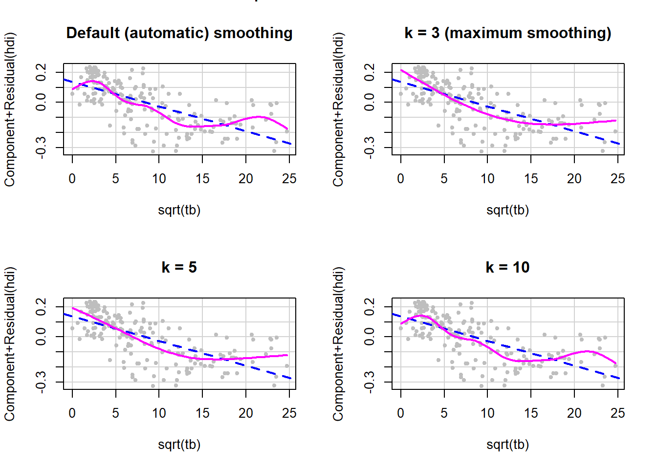
Figure 5.35: Changing the amount of smoothing in a CR plot
In this example, the default gives us a hint that there is non-linearity, but by smoothing more we see that it looks like a quadratic curve may be adequate. Note that adding a quadratic term in this example means adding the square of the square root, which is just tb itself, resulting in a model with both sqrt(tb) and tb. This will be explored in one of the exercises at the end of this chapter.