9.10 Regression diagnostics after MI
In previous chapters, various assumption checking and diagnostics were discussed for each type of regression model. How do we diagnose the fit of a model after MI? Any visual diagnostic plot can be examined within each imputation individually and compared between imputations. Also, diagnostic statistics can be computed within each imputation and pooled, for example, using pool.scalar(), micombine.chisquare(), or micombine.F() (the latter two from the miceadds package (Robitzsch, Grund, and Henke 2024)).
Two examples will be demonstrated here: visually checking linearity for a continuous predictor in a linear regression model and carrying out a Hosmer-Lemeshow goodness-of-fit test for a logistic regression model.
9.10.1 Example: Examining a diagnostic plot across imputations
As described in Section 5.17, use a CR plot to check the linearity assumption of a linear regression model. Display the plot for each imputation to get a visual assessment of the adequacy of the linearity assumption. For the linear regression model fit in Section 9.6, there were 20 imputations.
In practice, view all the plots for all continuous predictors. Here, for brevity, only the linearity assumption for one of the continuous predictors from Example 9.1 (BMXWAIST) is assessed and only for the first four imputations. As shown in Figure 9.7, the linearity assumption appears to be consistently met.
# To view for all imputations
# for(i in 1:length(fit.imp.lm$analyses)) {
#    Insert car::crPlots call here
# }

# Just the first four imputations
par(mfrow=c(2,2))
for(i in 1:4) {
  car::crPlots(fit.imp.lm$analyses[[i]],
               terms = ~ BMXWAIST,
               pch=20, col="gray",
               smooth = list(smoother=car::gamLine),
               ylab = "Comp + Resid",
               # In general, no need to specify ylim.
               # It is included here because outliers
               # make it harder to see patterns on the
               # the original scale, so zooming in helps.
               ylim = c(-0.05, 0.05))
}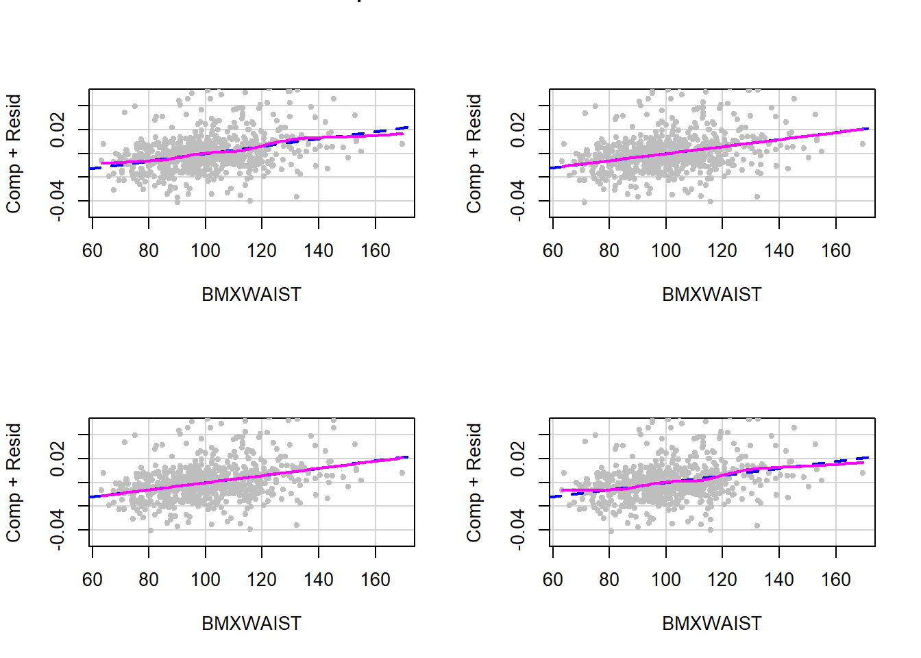
Figure 9.7: Checking the linearity assumption within each imputation
9.10.2 Example: Pooling a diagnostic test over imputations
The Hosmer-Lemeshow goodness-of-fit test computes a chi-squared statistic. Compute this statistic on the fit to each imputed dataset, and then use micombine.chisquare() (Li et al. 1991; Enders 2010) to pool over imputations. Although, in this example, the individual tests are chi-square tests, after pooling the over imputations the test turns out to be an F test.
# Initialize a vector to store the chi-squared values
X2 <- rep(NA, length(fit.imp.glm$analyses))

# Compute chi-squared statistic on each imputation
# (and store the degrees of freedom, as well)
for(i in 1:length(X2)) {
  HL <- ResourceSelection::hoslem.test(fit.imp.glm$analyses[[i]]$y,
                                       fit.imp.glm$analyses[[i]]$fitted.values)
  X2[i] <- HL$statistic # Chi-squared value
  DF    <- HL$parameter # Degrees of freedom
  rm(HL)
}

# Input the chi-squared vector and the degrees of freedom
# to pool over imputations
micombine.chisquare(X2, DF)
## Combination of Chi Square Statistics for Multiply Imputed Data
## Using 20 Imputed Data Sets
## F(8, 163.64)=0.321 p=0.9571