7.23 Writing it up
This section demonstrates how to write up the Cox regression methods and results for Example 7.6, first for a model assuming PH (cox.ex7.6), followed by a model that relaxes the PH assumption (cox.ex7.6.tt2). By way of reminder, Example 7.6 was: Using the Natality teaching dataset, estimate the association between previous preterm birth (RF_PPTERM) and time to preterm birth, adjusted for mother’s age (MAGER), race/ethnicity (MRACEHISP), and marital status (DMAR).
7.23.1 Writing up Cox regression results (assuming PH)
Below are a few lines of code to extract the information we need for our write-up.
Outcome, predictors, and dataset name
## coxph(formula = Surv(gestage37, preterm01) ~ RF_PPTERM + MAGER +
##     MRACEHISP + DMAR, data = natality.complete)
Number of observations: If we used a complete case analysis, then the number of rows in the dataset (nrow(natality.complete)) is the number of cases used in the analysis. But counting the number of residuals to get the sample size will work even when you have missing data.
## [1] 1743Selected descriptives: Extract any descriptive summaries you might want to add to your write-up. For example, the distribution of ages or the proportion of individuals in each race/ethnicity group. If you did not remove missing data first before fitting the model, do that here before creating any summary statistics. We want our summary to be based on the same sample as our regression model, and a regression will always carry out a complete case analysis whether you removed the cases with missing values first or not.
# Distribution of ages
c(
  min(natality.complete$MAGER),
  max(natality.complete$MAGER),
  mean(natality.complete$MAGER),
  sd(natality.complete$MAGER)
)
## [1] 15.000 49.000 28.964 5.817# Number and proportion for previous preterm
rbind(
table(natality.complete$RF_PPTERM),
round(100*prop.table(table(natality.complete$RF_PPTERM)), 1)
)## No Yes
## [1,] 1683.0 60.0
## [2,] 96.6 3.4# Number and proportion for race/ethnicity
rbind(
table(natality.complete$MRACEHISP),
round(100*prop.table(table(natality.complete$MRACEHISP)), 1)
)## NH White NH Black NH Other Hispanic
## [1,] 961.0 291.0 141.0 350.0
## [2,] 55.1 16.7 8.1 20.1# Number and proportion for marital status
rbind(
table(natality.complete$DMAR),
round(100*prop.table(table(natality.complete$DMAR)), 1)
)## Married Unmarried
## [1,] 1088.0 655.0
## [2,] 62.4 37.6# Number and proportion of events
rbind(
table(natality.complete$preterm01),
round(100*prop.table(table(natality.complete$preterm01)), 1)
)## 0 1
## [1,] 1525.0 218.0
## [2,] 87.5 12.5# If S(t) dropped below 0.50, you could get the median time to preterm birth
tmp <- survfit(Surv(gestage37, preterm01) ~ 1, data = natality.complete)
summary(tmp)$table[c("median", "0.95LCL", "0.95UCL")]## median 0.95LCL 0.95UCL
## NA NA NA# If median survival time is missing, you could instead compute
# the median among those with the event
median(natality.complete$gestage37[natality.complete$preterm01 == 1])## [1] 35Individual term regression coefficients, p-values, AHRs, and 95% confidence intervals: The p-value for the regression coefficients for a continuous predictor tests the association between that predictor and the outcome. For categorical predictors, each p-value is for a test comparing the hazard of the outcome between the level shown in that row and the reference level.
# Regression coefficients and 95% CIs
cbind("Beta" = summary(cox.ex7.6)$coef[, "coef"],
      confint(cox.ex7.6))
# (results not shown)
# AHRs, 95% CIs, p-values
cbind("AHR" = exp(summary(cox.ex7.6)$coef[, "coef"]),
exp(confint(cox.ex7.6)),
"p-value" = summary(cox.ex7.6)$coef[, "Pr(>|z|)"])
# (results not shown)Type III test p-values: For continuous predictors and categorical predictors with exactly two levels, the Type III Wald test p-values are the same as those in the regression coefficient table. For categorical predictors with more than two levels, Type III tests provide the multiple degree of freedom p-values for the overall test of that predictor’s association with the outcome (unless there is an interaction in the model, in which case the main effect test assumes the other term in the interaction is 0 or at its reference level).
# Multiple df p-values
car::Anova(cox.ex7.6, type = 3, test.statistic = "Wald")
# (results not shown)
Methods: We used data from 1743 births from a teaching dataset based on a modified subset of the 2019 US Natality data, including gestational age and an indicator of preterm birth (gestational age < 37 weeks). Cox proportional hazards regression was used to assess the association between previous preterm birth and the hazard of preterm birth, adjusted for mother’s age, race/ethnicity (non-Hispanic White, non-Hispanic Black, non-Hispanic Other, and Hispanic), and marital status (married, unmarried). Gestational ages \(\geq\) 37 weeks were censored at 37 weeks. We assessed the linearity and proportional hazards assumptions and checked for separation, collinearity, outliers, and influential observations (no issues were found). (In fact, we did find non-proportional hazards, and the corresponding write-up is shown below.)
Results: There were 218 preterm births (12.5%). Among these, the median gestational age was 35 weeks. Mothers were age 15 to 49 years (mean = 29.0, SD = 5.8), the majority were married (62.4%) and non-Hispanic White (NH White = 55.1%, NH Black = 16.7%, NH Other = 8.1%, Hispanic = 20.1%). A total of 60 (3.4%) mothers had a previous preterm birth. After adjusting for mother’s age, race/ethnicity, and marital status, previous preterm birth was significantly positively associated with preterm birth (AHR = 2.89; 95% CI = 1.82, 4.60; p <.001). Those with a previous preterm birth have 2.89 times the hazard of preterm birth. Mother’s age, race/ethnicity, and marital status were each also significantly associated with preterm birth, with older, non-Hispanic Black, and unmarried mothers having greater hazard.
See Table 7.2 for full regression results. Once again, use tbl_regression() to produce a nice looking table.
NOBS <- length(cox.ex7.6$residuals)

library(gtsummary)
# Table of regression coefficients
t1 <- cox.ex7.6 %>%
  tbl_regression(estimate_fun = function(x) style_number(x, digits = 2),
                 label  = list(RF_PPTERM  ~ "Previous Pre-Term",
                               MAGER      ~ "Age (y)",
                               MRACEHISP  ~ "Race/Ethnicity",
                               DMAR       ~ "Marital Status")) %>%
  modify_column_hide(p.value) %>%
  modify_caption(paste("Cox regression results for time to preterm birth vs.
                       previous preterm birth (N = ", NOBS, ")", sep=""))

# Table of hazard ratios
t2 <- cox.ex7.6 %>%
  tbl_regression(exponentiate = T,  # HR = exp(B)
                 estimate_fun = function(x) style_number(x, digits = 2),
                 pvalue_fun   = function(x) style_pvalue(x, digits = 3),
                 label  = list(RF_PPTERM  ~ "Previous Pre-Term",
                               MAGER      ~ "Age (y)",
                               MRACEHISP  ~ "Race/Ethnicity",
                               DMAR       ~ "Marital status")) %>%
  add_global_p(keep = T, test = "Wald")
TABLE <- tbl_merge(
tbls = list(t1, t2),
tab_spanner = c("**Adjusted Coefficient**", "**Adjusted Hazard Ratio**")
) %>%
modify_footnote(everything() ~ NA, abbreviation = TRUE) %>%
modify_header(update = list(
estimate_1 = "**log(AHR)**",
estimate_2 = "**AHR**"
))| Characteristic |
Adjusted Coefficient
|
Adjusted Hazard Ratio
|
|||
|---|---|---|---|---|---|
| log(AHR) | 95% CI | AHR | 95% CI | p-value | |
| Previous Pre-Term | <0.001 | ||||
| No | — | — | — | — | |
| Yes | 1.06 | 0.60, 1.53 | 2.89 | 1.82, 4.60 | <0.001 |
| Age (y) | 0.03 | 0.01, 0.05 | 1.03 | 1.01, 1.06 | 0.009 |
| Race/Ethnicity | 0.013 | ||||
| NH White | — | — | — | — | |
| NH Black | 0.56 | 0.21, 0.91 | 1.75 | 1.23, 2.48 | 0.002 |
| NH Other | -0.07 | -0.65, 0.51 | 0.93 | 0.52, 1.66 | 0.804 |
| Hispanic | 0.26 | -0.09, 0.61 | 1.30 | 0.91, 1.84 | 0.146 |
| Marital Status | |||||
| Married | — | — | |||
| Unmarried | 0.58 | 0.28, 0.89 | |||
| Marital status | <0.001 | ||||
| Married | — | — | |||
| Unmarried | 1.79 | 1.33, 2.42 | <0.001 | ||
| Abbreviations: CI = Confidence Interval, HR = Hazard Ratio, NA | |||||
7.23.2 Writing up Cox regression results (relaxing PH)
There was one predictor (DMAR) that had both significantly non-proportional hazards and a visualization that indicated a meaningful deviation from PH. The model that included its interaction with time was cox.ex7.6.tt2. Extract the components needed from that model for the write-up. Also, re-use the AHR vs. time figure created in Section 7.16.3.
# Regression coefficients and 95% CIs
cbind("Beta" = summary(cox.ex7.6.tt2)$coef[, "coef"],
      confint(cox.ex7.6.tt2))
# (results not shown)
# AHRs, 95% CIs, p-values
cbind("AHR" = exp(summary(cox.ex7.6.tt2)$coef[, "coef"]),
exp(confint(cox.ex7.6.tt2)),
"p-value" = summary(cox.ex7.6.tt2)$coef[, "Pr(>|z|)"])
# (results not shown)Methods: (Same as above, but with the following addition.) We checked the PH assumption statistically and numerically. For predictors with a meaningfully large deviation from PH, we relaxed the assumption by including an interaction with time.
Results: (Same descriptives as above, but regression results are different.) In the adjusted model, due to a failure of the PH assumption, the effect of marital status was allowed to vary linearly with time. After adjusting for mother’s age, race/ethnicity, and marital status, previous preterm birth was significantly positively associated with preterm birth (AHR = 2.87; 95% CI = 1.81, 4.57; p <.001). Those with a previous preterm birth have 2.87 times the hazard of preterm birth. Mother’s age and race/ethnicity were each also significantly associated with preterm birth, with older and non-Hispanic Black mothers having greater hazard. Marital status had a significant interaction with time: unmarried mothers had greater hazard of preterm birth than married mothers, even more so earlier in pregnancy.
See Table 7.3 for full regression results.
# Table of regression coefficients
t1 <- cox.ex7.6.tt2 %>%
  tbl_regression(estimate_fun = function(x) style_number(x, digits = 2),
                 label  = list(RF_PPTERM  ~ "Previous Pre-Term",
                               MAGER      ~ "Age (y)",
                               MRACEHISP  ~ "Race/Ethnicity",
                               Unmarried     ~ "Unmarried",
                               # Have to use `name` since the name has a ( in it
                               `tt(Unmarried)` ~ "Unmarried x Time")) %>%
  modify_column_hide(p.value) %>%
  modify_caption(paste("Cox regression results for time to preterm birth vs.
                       previous preterm birth (N = ", NOBS, ")", sep=""))

# Table of hazard ratios
t2 <- cox.ex7.6.tt2 %>%
  tbl_regression(exponentiate = T,  # HR = exp(B)
                 estimate_fun = function(x) style_number(x, digits = 2),
                 pvalue_fun   = function(x) style_pvalue(x, digits = 3),
                 label  = list(RF_PPTERM  ~ "Previous Pre-Term",
                               MAGER      ~ "Age (y)",
                               MRACEHISP  ~ "Race/Ethnicity",
                               Unmarried     ~ "Unmarried",
                               `tt(Unmarried)` ~ "Unmarried x Time")) %>%
  add_global_p(keep = T, test = "Wald")
TABLE <- tbl_merge(
tbls = list(t1, t2),
tab_spanner = c("**Adjusted Coefficient**", "**Adjusted Hazard Ratio**")
) %>%
modify_footnote(everything() ~ NA, abbreviation = TRUE) %>%
modify_header(update = list(
estimate_1 = "**log(AHR)**",
estimate_2 = "**AHR**"
))| Characteristic |
Adjusted Coefficient
|
Adjusted Hazard Ratio
|
|||
|---|---|---|---|---|---|
| log(AHR) | 95% CI | AHR | 95% CI | p-value | |
| Previous Pre-Term | <0.001 | ||||
| No | — | — | — | — | |
| Yes | 1.06 | 0.59, 1.52 | 2.87 | 1.81, 4.57 | <0.001 |
| Age (y) | 0.03 | 0.01, 0.05 | 1.03 | 1.01, 1.06 | 0.009 |
| Race/Ethnicity | 0.014 | ||||
| NH White | — | — | — | — | |
| NH Black | 0.56 | 0.21, 0.90 | 1.74 | 1.23, 2.47 | 0.002 |
| NH Other | -0.07 | -0.65, 0.51 | 0.93 | 0.52, 1.66 | 0.811 |
| Hispanic | 0.26 | -0.09, 0.61 | 1.30 | 0.91, 1.85 | 0.143 |
| Unmarried | 7.19 | 2.84, 11.54 | 1,327.08 | 17.06, 103,243.47 | 0.001 |
| Unmarried x Time | -0.19 | -0.32, -0.07 | 0.82 | 0.73, 0.94 | 0.003 |
| Abbreviations: CI = Confidence Interval, HR = Hazard Ratio, NA | |||||
The very large AHR value for the Unmarried main effect is actually an extrapolation to \(t\) = 0 weeks, a time at which there were no events. In fact, there were no events prior to \(t\) = 17 weeks. Had we centered \(t\), for example at 30 weeks (e.g., tt = function(x, t, ...) x*(t - 30)) then the AHR for the main effect (Unmarried) would be much smaller. See Figure 7.25 for a visualization of how the marital status effect changes over time.
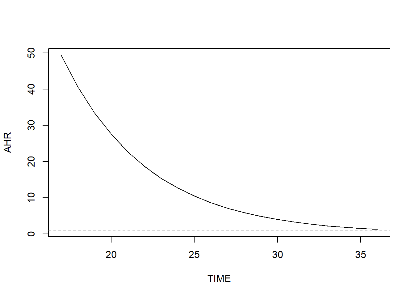
Figure 7.25: Preterm birth AHR for marital status (unmarried vs. married) vs. weeks (non-proportional hazards)