6.12 Assumptions

As with MLR, logistic regression assumes the observations are independent and this is checked in the same way as described in Section 5.14.

Unlike MLR, the logistic regression model does not include an error term (\(\epsilon\)). While it is possible to compute various kinds of residuals in a logistic regression, there is no assumption that they be normally distributed or have constant variance. Like MLR, however, logistic regression assumes that continuous predictors have a linear relationship with the outcome (in this case, with the log-odds of the probability of the outcome). Use a CR plot to diagnose non-linearity (see Section 5.16.2).

Example 6.3 (continued): Assess the linearity assumption in the adjusted model without an interaction.

# Enter just the continuous predictors in terms,
# separated by + signs. In this case, there is only one.
car::crPlots(fit.ex6.3.adj, terms = ~alc_agefirst,
             pch=20, col="gray",
             smooth = list(smoother=car::gamLine))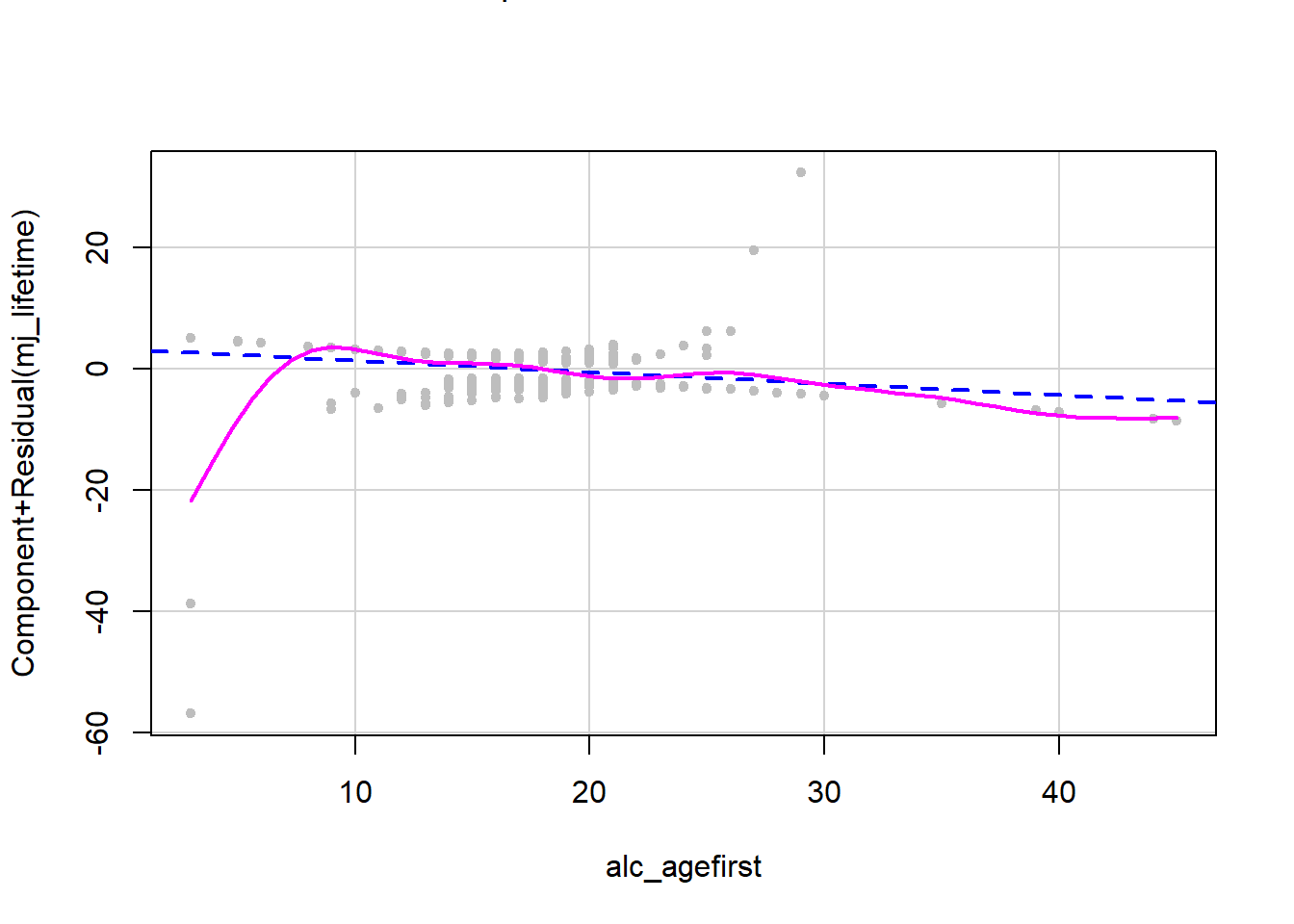

Figure 6.5: Component + residual plot for a continuous predictor in a logistic regression

# # If you want to try more smoothing change k
# car::crPlots(fit.ex6.3.adj, terms = ~alc_agefirst,
#              pch=20, col="gray",
#              smooth = list(smoother=car::gamLine, k = 5))

Figure 6.5 displays the CR plot for alc_agefirst. In a logistic regression, since the outcome can only take on two values, there will typically be a strong pattern in the points, but for diagnosis of non-linearity just focus on the dashed and solid lines. The dashed line illustrates the relationship between the continuous predictor and the outcome assuming linearity, while the solid line relaxes the linearity assumption. If these two are very different, then consider modeling the predictor using a non-linear function (e.g., adding a quadratic term, using a log or other non-linear transformation). In a logistic regression, make sure to only transform predictors, not the outcome.

Conclusion: There is no strong non-linearity. The dip in the solid line at lower ages of first alcohol use is in an area with few points so can be ignored – smoothers are highly influenced by local fluctuations.