5.22 Outliers
While collinearity diagnostics look for problems in the regression model due to relationships between predictors, outlier (this section) and influence (next section) diagnostics look for problems due to individual observations (cases).
An outlier is an individual observation with a very large residual. “Large” here means large in magnitude – either very positive or very negative residuals could be outliers. Outliers are not necessarily extreme in either the outcome (\(Y\)) or any of the predictors (\(X\)). What makes an observation an outlier in regression is that the observed value is far from the predicted value. For example, in the top left panel in Figure 5.46, the filled-in point is extreme in both the \(X\) and \(Y\) directions but is close to the line; therefore, its residual is small and it is not a regression outlier. In the top right and bottom left panels, the filled-in point has a typical \(X\) or \(Y\) value, respectively, but is an outlier since it is far from the line. In the bottom right panel, the point is extreme in both the \(X\) and \(Y\) directions and is far from the line, but what makes it an outlier is being far from the line.
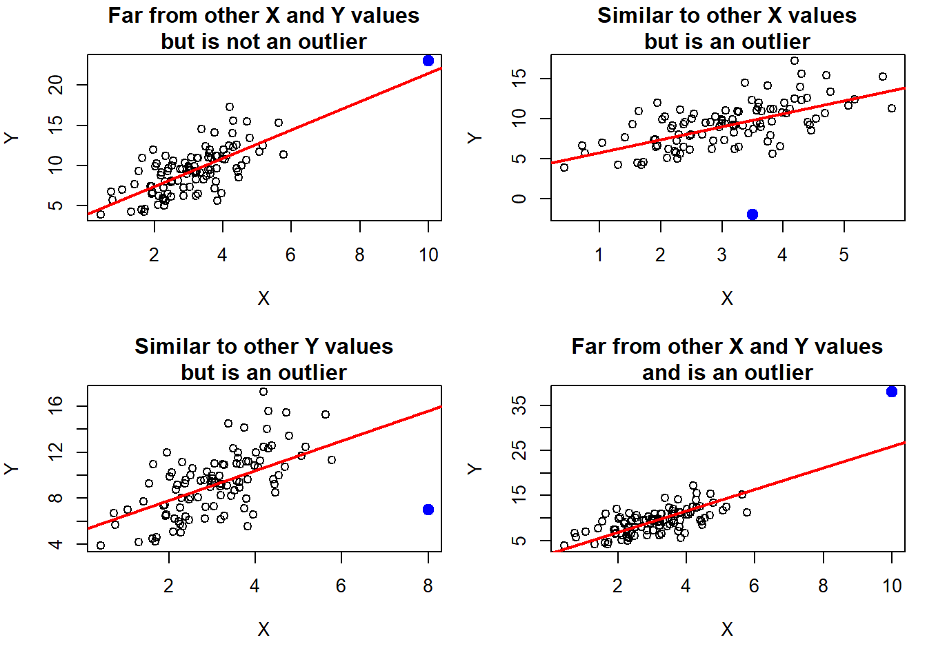
Figure 5.46: What is an outlier?
5.22.1 Impact of outliers
The presence of outliers can impact the validity of the normality and constant variance assumptions, resulting in invalid confidence intervals and p-values for regression coefficients. With a large sample size, these impacts will likely be small. Some outliers are also influential observations, a topic that will be discussed in Section 5.23. Finally, outliers are observations that are not well predicted by the model. Therefore, investigation of their characteristics may lead to new insights.
5.22.2 Diagnosis of outliers
We used Figure 5.46 to diagnose the presence of outliers in SLRs using outcome vs. predictor plots. In MLR, since there are multiple predictors, we instead detect outliers by looking at a plot of residuals vs. fitted values. Outliers are observations with large positive or negative residuals. How large is large enough to be considered an outlier? Recall that Studentized residuals have a \(t\) distribution (which approaches a standard normal distribution as the sample size increases). The cutoff for “large” is arbitrary, but we know that standard normal values larger in absolute value than 3 or 4 are very rare. They are less rare in larger samples, however, so we need a cutoff that changes with the sample size.
To diagnose and visualize outliers, we will (a) conduct a statistical test for outliers and (b) highlight the outliers in a plot of Studentized residuals vs. fitted values.
Example 5.1 (continued): Look for outliers in the model with the Box-Cox transformed outcome (fit.ex5.1.trans).
We start by carrying out a statistical test for outliers using car::outlierTest() (Fox, Weisberg, and Price 2024; Fox and Weisberg 2019). This tests each Studentized residual to see how likely we are to observe such an extreme value if the errors were truly \(t\) distributed. While large outliers are rare, they are less rare in larger samples. Therefore, a Bonferroni adjustment (see Section 5.25) is used to account for the increased chance of observing rare outcomes in larger samples. Observations are considered outliers if their Bonferroni p is <.05.
# Outlier test
# The default for n.max is 10. Using Inf leads to
# showing all the outliers if there are more than 10
car::outlierTest(fit.ex5.1.trans, n.max = Inf)
## rstudent unadjusted p-value Bonferroni p
## 1816 -11.808 0.000000000000000000000000000006887 0.000000000000000000000000005902
## 66 -5.408 0.000000082820999999999997624039461 0.000070976999999999994847392493
## 66.1 -5.408 0.000000082820999999999997624039461 0.000070976999999999994847392493Three observations were flagged by this test as having unusually large negative residuals, indicating that their observed fasting glucose values are much lower than predicted by the model. After adjusting for multiple testing, these three had Bonferroni p-values \(<\) .05. We will discuss multiple testing in Section 5.25 – for now just know that the Bonferroni adjustment accounts for the fact that in a large sample size, we might expect a few really extreme outliers, so an adjustment is needed to make sure we only flag really, really extreme ones.
NOTE: A car::outlierTest() Bonferroni p value of NA corresponds to non-significance.
The row labels in the outlier test output can be used to identify the outlying observations. Make sure to put them in quotes when subsetting the data (these are row labels, not row numbers).
nhanesf.complete[c("1816", "66", "66.1"),
                 c("LBDGLUSI", "BMXWAIST", "smoker",
                   "RIDAGEYR", "RIAGENDR", "race_eth", "income")]
## LBDGLUSI BMXWAIST smoker RIDAGEYR RIAGENDR race_eth income
## 1816 2.61 83.5 Past 59 Female Non-Hispanic Other $55,000+
## 66 3.50 110.5 Never 52 Female Non-Hispanic White $55,000+
## 66.1 3.50 110.5 Never 52 Female Non-Hispanic White $55,000+NOTE: Two of these rows are identical; this is an artifact of how the NHANES teaching datasets used in this book were created – by sampling with replacement from the full NHANES dataset (see Appendix A.1).
What makes these observations unusual? Looking at the regression coefficients below, we see that both age and waist circumference have positive associations with fasting glucose, and that past smokers have greater mean (transformed) fasting glucose. Looking at the overall distribution of the outcome and continuous predictors below, we see that these individuals have very low fasting glucose (LBDGLUSI), but some predictor values indicative of greater fasting glucose. For example, individual 1816 is a past smoker with above average age, and the other two individuals have above average waist circumference and above average age.
##                            Estimate Std. Error  t value Pr(>|t|)
## (Intercept)                  0.5874     0.0025 235.3593   0.0000
## BMXWAIST                     0.0002     0.0000   9.7339   0.0000
## smokerPast                   0.0012     0.0008   1.4326   0.1523
## smokerCurrent               -0.0001     0.0010  -0.0764   0.9391
## RIDAGEYR                     0.0002     0.0000   9.7597   0.0000
## RIAGENDRFemale              -0.0031     0.0007  -4.4107   0.0000
## race_ethNon-Hispanic White  -0.0030     0.0010  -3.0713   0.0022
## race_ethNon-Hispanic Black  -0.0017     0.0013  -1.3146   0.1890
## race_ethNon-Hispanic Other  -0.0005     0.0014  -0.3178   0.7507
## income$25,000 to <$55,000    0.0004     0.0011   0.3809   0.7034
## income$55,000+ -0.0001 0.0010 -0.0679 0.9459rbind(
"Glucose" = summary(nhanesf.complete$LBDGLUSI),
"Waist" = summary(nhanesf.complete$BMXWAIST),
"Age" = summary(nhanesf.complete$RIDAGEYR)
)## Min. 1st Qu. Median Mean 3rd Qu. Max.
## Glucose 2.61 5.33 5.72 6.11 6.22 19.0
## Waist 63.20 88.30 98.30 100.82 112.20 169.5
## Age 20.00 34.00 47.00 47.79 61.00 80.0You can visualize the outliers by highlighting them in a plot of Studentized residual vs. fitted values (Figure 5.47). To do this, we need a pair of cutoffs above and below which, respectively, are the residuals for the outliers identified by the outlier test (or just one cutoff if all the outliers are positive or all are negative). This can get tricky due to rounding, but just fiddle with the cutoffs until you get the right number of points highlighted in your plot. Again, due to the way this dataset was created, two of the outliers are identical so it will appear that only two points are highlighted since one is on top of the other.
# Compute Studentized residuals
RSTUDENT <- rstudent(fit.ex5.1.trans)

# Cutoff for flagging outliers based on the outlier test
SUB <- RSTUDENT < -5.38

# Check that you flagged the right number of outliers
sum(SUB)
## [1] 3# Plot Studentized residuals vs. fitted values
car::residualPlots(fit.ex5.1.trans,
pch=20, col="gray",
fitted = T, terms = ~ 1,
tests = F, quadratic = F,
type = "rstudent")
# Highlight outliers
# NOTE: For points() the arguments are x, y not y ~ x
points(fitted(fit.ex5.1.trans)[SUB], RSTUDENT[SUB], pch=20, cex=2)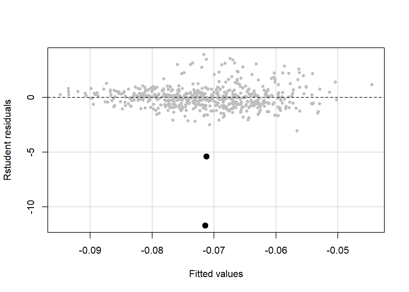
Figure 5.47: Highlighting outliers in a residual vs. fitted plot
NOTE: In this example, there were not any positive outliers. But, if there were, you would need to modify SUB above as in the examples below.
# Example 1: Suppose all the outliers have positive residuals with
#            the smallest being 4.62483
SUB <- RSTUDENT > 4.62

# Example 2: Suppose there are both positive and negative outliers
#            and, among the positive outliers, the smallest is 4.62483
#            and, among the negative outliers, the largest is -4.89398
SUB <- RSTUDENT > 4.62 | RSTUDENT < -4.89
5.22.3 Potential solutions for outliers
It is tempting to simply remove outliers. However, being an outlier does not alone justify removal of an observation. Removing outliers may make your model appear to fit better than it should, leading to overconfidence in your results. Given a set of observations with very large residuals, first check to see if the observed outcome and/or predictor values for those observations are data entry errors (if you have access to the raw data). If that is not possible, or if you have determined they are not data entry errors, then try one of the following options.
- Outcome transformation: If the \(Y\) distribution is very skewed, that can lead to large residuals. A transformation may solve this problem.
- Perform a sensitivity analysis: Fit the model with and without the outliers and see what changes (see Section 5.26). If the sample size is large, outliers will have little impact on your conclusions. But since there is no objective cutoff for “large” it is difficult to know if the outliers actually have little impact without carrying out a sensitivity analysis.
Finally, rather than simply being a problem, outliers may actually be some of the more interesting observations in the data. Observations that are not fit well by the model may warrant further investigation, possibly leading to new insights and hypotheses.