7.12 Interactions
As with linear and logistic regression, include interactions in a Cox model to assess effect modification. Including an interaction allows you to assess if the association between a risk factor and time to an event depends on another variable, and to estimate the HR for one variable at different levels of another.
Example 7.7: Using the Natality teaching dataset, see if the association between previous preterm birth and time to preterm birth (adjusted for age, race/ethnicity, and marital status) depends on whether or not the mother had pre-pregnancy hypertension (RF_PHYPE). As with any model with an interaction, include both the main effects and the interaction term.
cox.ex7.7.int <- coxph(Surv(gestage37, preterm01) ~ MAGER + MRACEHISP + DMAR +
                         RF_PPTERM + RF_PHYPE +  # Main effects
                         RF_PPTERM:RF_PHYPE,     # Interaction
                       data = natality)

round(
  cbind("AHR"      = exp(summary(cox.ex7.7.int)$coef[, "coef"]),
                     exp(confint(cox.ex7.7.int)),
        "p-value"  = summary(cox.ex7.7.int)$coef[, "Pr(>|z|)"])
  , 3)
## AHR 2.5 % 97.5 % p-value
## MAGER 1.032 1.008 1.057 0.009
## MRACEHISPNH Black 1.699 1.194 2.416 0.003
## MRACEHISPNH Other 0.929 0.520 1.657 0.802
## MRACEHISPHispanic 1.304 0.918 1.852 0.139
## DMARUnmarried 1.785 1.320 2.413 0.000
## RF_PPTERMYes 2.660 1.634 4.328 0.000
## RF_PHYPEYes 1.287 0.526 3.148 0.580
## RF_PPTERMYes:RF_PHYPEYes 6.774 1.195 38.392 0.031The interaction is statistically significant (the p-value for the RF_PPTERMYes:RF_PHYPEYes row is .031). Had either of the terms in the interaction been categorical with more than two levels, we would have used car::Anova(cox.ex7.7.int, type = 3, test = "Wald") to get the interaction p-value, as it would have been a multiple degree of freedom test.
7.12.1 Overall test of a predictor involved in an interaction
As shown in Section 5.10.11, we can also carry out an overall test of previous preterm birth by comparing the full model to the model with both the main effect (RF_PPTERM) and interaction (RF_PPTERM:RF_PHYPE) removed. We did not remove missing data prior to fitting the full model, so we need to create a dataset with no missing data first so both models can be fit to the same observations, or use the subset option. As with MLR, use anova() to compare the models but for a Cox regression we must specify test = "Chisq" to get a p-value. There is no option to specify a Wald test in this case; anova() uses a likelihood ratio test when comparing Cox models.
# Fit the reduced model using the subset option
# to remove missing values for the variable
# being removed to create the reduced model
fit0 <- coxph(Surv(gestage37, preterm01) ~
                   MAGER + MRACEHISP + DMAR +
                   RF_PHYPE,
              data = natality,
              subset = complete.cases(RF_PPTERM))
# Compare to full model
anova(fit0, cox.ex7.7.int, test = "Chisq")
## Analysis of Deviance Table
## Cox model: response is Surv(gestage37, preterm01)
## Model 1: ~ MAGER + MRACEHISP + DMAR + RF_PHYPE
## Model 2: ~ MAGER + MRACEHISP + DMAR + RF_PPTERM + RF_PHYPE + RF_PPTERM:RF_PHYPE
## loglik Chisq Df Pr(>|Chi|)
## 1 -1587
## 2 -1578 19.1 2 0.000071 ***
## ---
## Signif. codes: 0 '***' 0.001 '**' 0.01 '*' 0.05 '.' 0.1 ' ' 1The 2 df test (2 df because the models differ in two terms – the main effect and the interaction) results in a p-value that is very small. Thus, after adjusting for age, race/ethnicity, marital status, and pre-pregnancy hypertension, previous preterm birth is significantly associated with time to preterm birth.
7.12.2 Estimating the HR at each level of the other variable
In addition to the test of significance, we also would like to know what is the magnitude of the AHR for previous preterm birth among those with and without pre-pregnancy hypertension. The main effect for RF_PPTERM provides the AHR for previous preterm birth among those at the reference level of RF_PHYPE (“No”). For linear and logistic regression models, we used gmodels::estimable() to estimate the AHR at non-reference levels of the other predictor in the interaction. Unfortunately, gmodels::estimable() does not work for a coxph object. Instead, re-fit the model after changing the reference level of RF_PHYPE to “Yes” which will result in a main effect for RF_PPTERM at the new reference level. In this way, we can get the AHR, 95% CI, and p-value for RF_PPTERM at each level of RF_PHYPE.
First, using the original model, extract the results for the main effect RF_PPTERM, which is the effect at RF_PHYPE = “No” (the reference level for RF_PHYPE).
round(
  cbind("AHR"      = exp(summary(cox.ex7.7.int)$coef[, "coef"]),
                     exp(confint(cox.ex7.7.int)),
        "p-value"  = summary(cox.ex7.7.int)$coef[, "Pr(>|z|)"])["RF_PPTERMYes", ]
  , 3)
## AHR 2.5 % 97.5 % p-value
## 2.660 1.634 4.328 0.000Next, re-level RF_PHYPE (not RF_PPTERM), re-fit the model, and extract the main effect results again to get the RF_PPTERM effect at RF_PHYPE = “Yes”.
natality_b <- natality %>%
  mutate(RF_PHYPE = relevel(RF_PHYPE, ref = "Yes"))

# Re-fit with data = natality_b
cox.ex7.7.int_b <- coxph(Surv(gestage37, preterm01) ~
                   MAGER + MRACEHISP + DMAR +
                   RF_PPTERM + RF_PHYPE +
                   RF_PPTERM:RF_PHYPE,
                   data = natality_b)

round(
  cbind("AHR"      = exp(summary(cox.ex7.7.int_b)$coef[, "coef"]),
                     exp(confint(cox.ex7.7.int_b)),
        "p-value"  = summary(cox.ex7.7.int_b)$coef[, "Pr(>|z|)"])["RF_PPTERMYes",]
  , 3)
## AHR 2.5 % 97.5 % p-value
## 18.016 3.406 95.289 0.001The AHR for previous preterm birth is greater among those with pre-pregnancy hypertension (18.016) than among those without (2.660) (interaction p-value = .031, a test of the null hypothesis that these two AHRs are the same).
The AHR among those with pre-pregnancy hypertension is quite large and has a very wide CI. Why? It turns out that there were not many cases with pre-pregnancy hypertension, resulting in high variability when estimating the AHR in this subgroup and a wide CI.
##
##   No  Yes
## 1965   34
Also, among those with pre-pregnancy hypertension, only two mothers had a previous preterm birth and both experienced a preterm birth, which explains the large RF_PPTERM AHR in this group.
# Previous preterm vs. preterm
# among those with hypertension
table(natality$RF_PPTERM[natality$RF_PHYPE == "Yes"],
      natality$preterm01[natality$RF_PHYPE == "Yes"])
##
## 0 1
## No 27 5
## Yes 0 2You may have noticed that there is a 0 in this table. With logistic regression, a 0 in the two-way table comparing a categorical predictor to the outcome was an indication that logistic regression would have convergence problems due to separation (Section 6.10). In Section 7.13 we will discuss this same issue in the context of a Cox regression model. It turns out this particular 0 does not cause a problem with separation, but others will.
7.12.3 Visualizing an interaction
Plot the survival functions illustrating the previous preterm birth effect among those without and with pre-pregnancy hypertension. The code is similar to that in Section 7.11, but now we need a data.frame for each combination of levels of RF_PPTERM and RF_PHYPE.
# RF_PPTERM = "Yes", RF_PHYPE  = "Yes"
DAT_PPTERM_Yes_PHYPE_Yes <- data.frame(
            preterm01 = 1,
            gestage37 = 17:36,
            DMAR      = "Married",
            MRACEHISP = "NH White",
            MAGER     = mean(natality.complete$MAGER),
            RF_PPTERM = "Yes",
            RF_PHYPE  = "Yes")

# Other three combinations
# Copy first data.frame
DAT_PPTERM_Yes_PHYPE_No <- DAT_PPTERM_Yes_PHYPE_Yes
DAT_PPTERM_No_PHYPE_Yes <- DAT_PPTERM_Yes_PHYPE_Yes
DAT_PPTERM_No_PHYPE_No  <- DAT_PPTERM_Yes_PHYPE_Yes

# Update values of the 2 terms in the interaction
DAT_PPTERM_Yes_PHYPE_No$RF_PPTERM <- "Yes"
DAT_PPTERM_Yes_PHYPE_No$RF_PHYPE  <- "No"

DAT_PPTERM_No_PHYPE_Yes$RF_PPTERM <- "No"
DAT_PPTERM_No_PHYPE_Yes$RF_PHYPE  <- "Yes"

DAT_PPTERM_No_PHYPE_No$RF_PPTERM <- "No"
DAT_PPTERM_No_PHYPE_No$RF_PHYPE  <- "No"
When computing the predictions, be careful to use the original fit for the combinations with RF_PHYPE = “No” (the original reference level of the other term in the interaction) and the re-leveled fit for RF_PHYPE = “Yes” (the reference level after re-leveling).
# Predictions
# Use re-leveled fit when RF_PHYPE = "Yes" (ref level after re-leveling)
PRED_PPTERM_Yes_PHYPE_Yes <-
  predict(cox.ex7.7.int_b, DAT_PPTERM_Yes_PHYPE_Yes, type = "survival")

# Use original fit when RF_PHYPE = "No" (original ref level)
PRED_PPTERM_Yes_PHYPE_No  <-
  predict(cox.ex7.7.int,   DAT_PPTERM_Yes_PHYPE_No,  type = "survival")

# Use re-leveled fit when RF_PHYPE = "Yes" (ref level after re-leveling)
PRED_PPTERM_No_PHYPE_Yes  <-
  predict(cox.ex7.7.int_b, DAT_PPTERM_No_PHYPE_Yes,  type = "survival")

# Use original fit when RF_PHYPE = "No" (original ref level)
PRED_PPTERM_No_PHYPE_No   <-
  predict(cox.ex7.7.int,   DAT_PPTERM_No_PHYPE_No,   type = "survival")
Finally, plot the predictions.
# RF_PHYPE = "No"
par(mfrow=c(1,2))
plot(0, 0, col = "white",
     xlab = "Gestational Age (weeks)", ylab = "P(Not yet preterm)",
     xlim = c(17, 36),
     ylim = c(0, 1),
     font.axis = 2, font.lab = 2,
     main = "Without hypertension")
# NOTE: For lines() the arguments are x, y not y ~ x
lines( DAT_PPTERM_No_PHYPE_No$gestage37,
      PRED_PPTERM_No_PHYPE_No,  lwd = 2, lty = 1)
lines( DAT_PPTERM_Yes_PHYPE_No$gestage37,
      PRED_PPTERM_Yes_PHYPE_No, lwd = 2, lty = 2)
legend(17, 0.55, c("No", "Yes"), title = "Previous preterm birth",
       lty=c(1,2), lwd=c(2,2), bty = "n")

# RF_PHYPE = "Yes"
plot(0, 0, col = "white",
     xlab = "Gestational Age (weeks)", ylab = "P(Not yet preterm)",
     xlim = c(17, 36),
     ylim = c(0, 1),
     font.axis = 2, font.lab = 2,
     main = "With hypertension")
# NOTE: For lines() the arguments are x, y not y ~ x
lines(DAT_PPTERM_No_PHYPE_Yes$gestage37,
      PRED_PPTERM_No_PHYPE_Yes,  lwd = 2, lty = 1)
lines(DAT_PPTERM_Yes_PHYPE_Yes$gestage37,
      PRED_PPTERM_Yes_PHYPE_Yes, lwd = 2, lty = 2)
legend(17, 0.55, c("No", "Yes"), title = "Previous preterm birth",
       lty=c(1,2), lwd=c(2,2), bty = "n")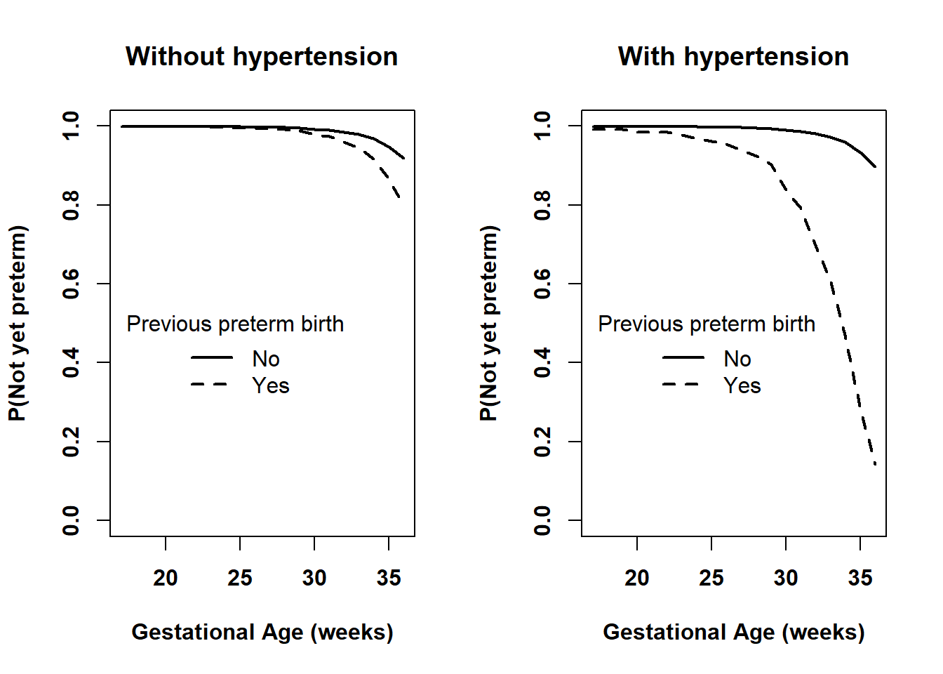
Figure 7.15: Comparing the survival functions between those without and with previous preterm birth at each level of pre-pregnancy hypertension
It is a good idea to compare the visualization of an interaction to the estimated AHR at each level of the other variable in the interaction. If they are not consistent, then the estimation and/or plotting code have an error. In Section 7.12.2, we estimated that the AHR for RF_PPTERM at RF_PHYPE = “No” is 2.660 and at RF_PHYPE = “Yes” is 18.016. These are consistent with Figure 7.15. Both AHRs are greater than 1 and in both plots the survival curve for RF_PPTERM = “Yes” is lower than that for “No”. Also, the AHR for RF_PPTERM at RF_PHYPE = “Yes” is much larger than at RF_PHYPE = “No” and the lines in the right panel are much further apart than those in the left panel.
The right panel in Figure 7.15 shows that, based on this dataset, we estimate that those with both a previous preterm birth and pre-pregnancy hypertension (and other predictors as specified above) have over 85% probability of preterm birth (the dashed survival function drops below 0.15). Be wary of this estimate, however, since, as seen above, it is based on a very small sample size. Using the methods from Section 7.10, compute a 95% CI for this quantity to get an idea of how imprecise it is.
unlist(summary(survfit(cox.ex7.7.int_b,
   DAT_PPTERM_Yes_PHYPE_Yes[DAT_PPTERM_Yes_PHYPE_Yes$gestage37 == 36,],
   se.fit =T, conf.int = 0.95),
 times=36)[c("surv", "std.err", "lower", "upper")])
## surv std.err lower upper
## 0.141915 0.204637 0.008407 1.000000Conclusion: After adjusting for mother’s age, race/ethnicity, marital status, and pre-pregnancy hypertension, previous preterm birth is significantly associated with time to preterm birth (p <.001 – from the test comparing the model with an interaction to the model with no RF_PPTERM main effect or interaction). The association between previous preterm birth and time to preterm birth differs significantly between those without and with pre-pregnancy hypertension (interaction p = .031). Among mothers who did not have pre-pregnancy hypertension, those with a previous preterm birth have 2.7 times the hazard of preterm birth of those who did not (AHR = 2.66; 95% CI = 1.63, 4.33; p <.001). Among those who did have pre-pregnancy hypertension, the hazard is even larger (AHR = 18.0; 95% CI = 3.4, 95.3; p <.001).