9.5 Descriptive statistics after MI
After MI, compute descriptive statistics within each complete dataset and use Rubin’s rules to pool statistics and compute their standard errors. Rubin’s rules comprise two parts – one for computing the statistic and one for its variation. For the statistic, simply average the values over the imputations. For the variation of the statistic, combine the average variance over imputations with the variation of the statistic between imputations. Additionally, if the sampling distribution of the statistic is not close to normal, then it is recommended to transform the statistic to normality before applying Rubin’s rules.
Statistics for which we can assume normality (in a large sample) include the mean and standard deviation of a continuous variable and the frequencies and proportions of levels of a categorical variable. A list of appropriate transformations for other statistics (e.g., correlation, odds ratio) can be found at Scalar inference of non-normal quantities (van Buuren 2018). The strategy in that case is to transform, apply Rubin’s rules, and then back-transform to the original scale.
Later, this section will introduce some convenient functions for computing descriptive statistics after MI. But first, we demonstrate how to use Rubin’s rules to compute the mean and standard error of the mean waist circumference from Example 9.1. To do this, extract the multiply imputed datasets, compute the sample mean and variance of the sample mean for waist circumference in each, and then combine them using Rubin’s rules to get the mean and standard error pooled over the imputations. Recall that the variance of the sample mean is the sample variance divided by the sample size.
# Multiple imputed datasets stacked together
# but NOT including the original data
imp.nhanes.dat <- complete(imp.nhanes.new, action = "long")

# Sample mean in each complete imputed dataset
MEAN     <- tapply(imp.nhanes.dat$BMXWAIST, imp.nhanes.dat$.imp, mean)

# Variance of the sample mean in each imputed dataset
# Make sure to use imp.nhanes.new (the mids object)
# inside nrow!
VAR.MEAN <- tapply(imp.nhanes.dat$BMXWAIST,
                   imp.nhanes.dat$.imp,
                   var) / nrow(imp.nhanes.new$data)
The following shows the means and variances by imputation, in a table and visually.
##     MEAN VAR.MEAN
## 1  100.3   0.2857
## 2  100.4   0.2834
## 3  100.4   0.2903
## 4  100.6   0.2826
## 5  100.5   0.2910
## 6  100.4   0.2860
## 7  100.4   0.2865
## 8  100.6   0.2896
## 9  100.5   0.2908
## 10 100.4   0.2835
## 11 100.6   0.2876
## 12 100.5   0.2882
## 13 100.3   0.2892
## 14 100.3   0.2894
## 15 100.4   0.2908
## 16 100.5   0.2878
## 17 100.4   0.2875
## 18 100.5   0.2888
## 19 100.4   0.2842
## 20 100.5 0.2866par(mfrow=c(1,2))
plot(MEAN ~ I(1:imp.nhanes$m),
ylab = "Mean", xlab = "Imputation",
main = "Mean\nby imputation")
abline(h=mean(MEAN), col="red", lty=2, lwd=2)
plot(VAR.MEAN ~ I(1:imp.nhanes$m),
ylab = "Variance of Mean", xlab = "Imputation",
main = "Variance of Mean\nby imputation")
abline(h=mean(VAR.MEAN), col="red", lty=2, lwd=2)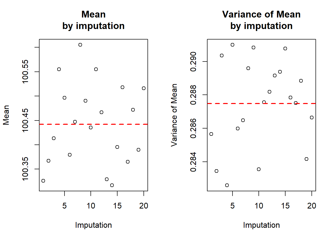
Figure 9.5: Mean and variance of waist circumference across multiple complete (imputed) datasets
The average of the 20 within-imputation sample means is 100.44 cm (the horizontal dashed line in the left panel of Figure 9.5) and is the correct estimate of the mean waist circumference. The average of the 20 within-imputation variances of the sample mean is 0.2875. This turns out to be an underestimate of the variance of the sample mean waist circumference. It needs to be increased based on how variable the means are between imputations. The Rubin’s rule formula for the pooled variance adds the average variance to a factor times the variance of the means. Below, the pool.scalar() function does the computations for us and the pooled mean and variance of the mean are manually computed, as well. The latter is just to illustrate what pool.scalar() is doing; in future, just use pool.scalar().
# Rubin's rules for the mean and variance of the mean
# Using pool.scalar()
POOLED <- pool.scalar(MEAN,
                      VAR.MEAN,
                      nrow(imp.nhanes.new$data))
data.frame(pooled.mean = POOLED$qbar,
           mean.var    = POOLED$ubar,
           btw.var     = POOLED$b,
           pooled.var  = POOLED$t)
## pooled.mean mean.var btw.var pooled.var
## 1 100.4 0.2875 0.007014 0.2948# Manually (just for illustration)
data.frame(pooled.mean = mean(MEAN),
mean.var = mean(VAR.MEAN),
btw.var = var(MEAN),
pooled.var = mean(VAR.MEAN) + (1 + 1/length(MEAN))*var(MEAN))## pooled.mean mean.var btw.var pooled.var
## 1 100.4 0.2875 0.007014 0.2948In this example, there was not much missing data, so there was not much variation in the means (the between-imputation variance, btw.var is small), so the pooled variance is not that much larger than the mean of the variances.
Finally, to get the pooled standard error of the mean, take the square root of the pooled variance of the mean.
## [1] 0.543NOTE: This is the pooled standard error of the mean. If you want the pooled standard deviation of waist circumference, average the within-imputation standard deviations over the imputations.
The steps of computing descriptive statistics (mean, standard error of the mean, and standard deviation for continuous variables; frequency and proportion for categorical variables) in each dataset and pooling using Rubin’s rules have been coded into the functions mi.mean.se.sd(), mi.n.p(), mi.mean.se.sd.by(), and mi.n.p.by() (found in Functions_rmph.R which you loaded at the beginning of this chapter). These operate directly on a mids object so there is no need to use complete() to convert to a data.frame first.
NOTES:
- For variables with no missing data, these
mi.functions will return the same values as standard descriptive statistic functions. - For frequencies of categorical variables that have missing values, the results after MI may not be whole numbers, as they are averages over imputations.
- If a “by” variable has missing values, then even frequencies for variables that did not have missing values may not be whole numbers, as the split between groups will differ between imputations.
Each function call returns a data.frame and rbind() stacks the results together.
# Means and standard deviations
rbind(mi.mean.se.sd(imp.nhanes.new, "LBDGLUSI"),
      mi.mean.se.sd(imp.nhanes.new, "BMXWAIST"),
      mi.mean.se.sd(imp.nhanes.new, "RIDAGEYR"))
## mean se sd
## LBDGLUSI 6.093 0.05096 1.611
## BMXWAIST 100.442 0.54299 16.955
## RIDAGEYR 47.876 0.52657 16.652# Frequencies and proportions
rbind(mi.n.p(imp.nhanes.new, "smoker"),
mi.n.p(imp.nhanes.new, "RIAGENDR"),
mi.n.p(imp.nhanes.new, "race_eth"),
mi.n.p(imp.nhanes.new, "income"))## n p
## smoker: Never 579.0 0.5790
## smoker: Past 264.0 0.2640
## smoker: Current 157.0 0.1570
## RIAGENDR: Male 457.0 0.4570
## RIAGENDR: Female 543.0 0.5430
## race_eth: Hispanic 191.0 0.1910
## race_eth: NH White 602.0 0.6020
## race_eth: NH Black 115.0 0.1150
## race_eth: NH Other 92.0 0.0920
## income: <$25,000 188.9 0.1889
## income: $25,000 to <$55,000 258.4 0.2584
## income: $55,000+ 552.7 0.5527# Means and standard deviations by another variable
rbind(mi.mean.se.sd.by(imp.nhanes.new, "LBDGLUSI", BY = "wc_median_split"),
mi.mean.se.sd.by(imp.nhanes.new, "RIDAGEYR", BY = "wc_median_split"))## mean.1 se.1 sd.1 mean.2 se.2 sd.2
## LBDGLUSI 5.701 0.05341 1.173 6.48 0.08404 1.871
## RIDAGEYR 44.594 0.76423 16.727 51.11 0.72326 15.943# Frequencies and proportions by another variable
rbind(mi.n.p.by(imp.nhanes.new, "smoker", BY = "wc_median_split"),
mi.n.p.by(imp.nhanes.new, "RIAGENDR", BY = "wc_median_split"),
mi.n.p.by(imp.nhanes.new, "race_eth", BY = "wc_median_split"),
mi.n.p.by(imp.nhanes.new, "income", BY = "wc_median_split"))## n.1 p.1 n.2 p.2
## smoker: Never 314.50 0.6336 264.50 0.52522
## smoker: Past 110.15 0.2219 153.85 0.30550
## smoker: Current 71.75 0.1445 85.25 0.16928
## RIAGENDR: Male 212.20 0.4275 244.80 0.48610
## RIAGENDR: Female 284.20 0.5725 258.80 0.51390
## race_eth: Hispanic 91.60 0.1845 99.40 0.19738
## race_eth: NH White 292.40 0.5890 309.60 0.61477
## race_eth: NH Black 57.15 0.1151 57.85 0.11487
## race_eth: NH Other 55.25 0.1113 36.75 0.07297
## income: <$25,000 83.55 0.1683 105.35 0.20919
## income: $25,000 to <$55,000 132.20 0.2663 126.20 0.25060
## income: $55,000+ 280.65 0.5654 272.05 0.54021