5.19 Box-Cox outcome transformation
Continuous variables that are highly skewed are common in public health. For example, any variable that is derived as the sum of multiple indicators will have all non-negative values and this often leads to a skewed distribution. For example, in Rogers et al. (2021), researchers log-transformed the skewed outcome variable frailty index (FI), derived as the sum of 34 indicators across a number of health domains, prior to fitting linear regression studying the association between childhood socioeconomic status and frailty. Due to the presence of zero values, they used the transformation \(\log(FI + 0.01)\). Other examples of skewed variables include population size, income, and costs. For example, in Sakai-Bizmark et al. (2021), researchers log-transformed cost of hospitalization in a linear regression investigating the association between homelessness and health outcomes in youth.
The previous sections included recommendations for handling assumption violations using variable transformations. The natural logarithm, square root, and inverse transformations are special cases of the more general Box-Cox family of transformations (Box and Cox 1964). Note that, as presented here, the method only applies to transformation of the outcome, not predictors. Also, the method assumes that the outcome values are all positive. If there are a few zero or negative values, a modification of the Box-Cox that allows non-positive values (Box-Cox with negatives, BCN) can be used (Hawkins and Weisberg 2017). If there are zero values, but no negative values, as mentioned previously an option is to add a small number before carrying out the transformation, although if there are a large number of zero values then it is possible no Box-Cox transformation will sufficiently normalize the errors or stabilize the variance of the errors.
Consider the family of transformations of a positive outcome \(Y\) defined by \((Y^{\lambda}-1) / \lambda\). The square root transformation is proportional to \(\lambda = 0.5\) and the inverse transformation to \(\lambda\) = –1. By convention, \(\lambda = 0\) corresponds to the natural log transformation. We will use MASS::boxcox() (Ripley and Venables 2025; Venables and Ripley 2002) to find the value of \(\lambda\) that optimally transforms the outcome \(Y\) for a linear regression model.
In summary,
- if \(\lambda\) is close to 1, then no transformation is needed; otherwise,
- if \(\lambda\) is close to 0, replace \(Y\) with \(\ln{(Y)}\); otherwise,
- replace \(Y\) with \((Y^{\lambda}-1) / \lambda\).
What is “close” to 1 or 0 is arbitrary. All else being equal, a model with no outcome transformation is most desirable as the results are easier to explain and all predictions are on the original scale. So unless \(\lambda\) is far enough from 1 to make a meaningful difference in the validity of the assumptions (e.g., constant variance is strongly violated), you might as well stick with no outcome transformation. Similarly, when a transformation is needed but \(\lambda\) is not far enough from 0 to make a meaningful difference, then use a log-transformation since it is commonly used and therefore understandable to a broader audience.
Example 5.1 (continued): In Sections 5.17 and 5.18 we found the following assumption violations:
- Possible non-linearity in waist circumference, and
- Non-constant variance of the errors – the variance was larger for observations with larger fitted values.
The Box-Cox method searches over a range of possible transformations and finds the optimal one. MASS::boxcox() produces a plot of the profile log-likelihood values (the definition of this term is beyond the scope of this text) as a function of \(\lambda\) (Figure 5.39).
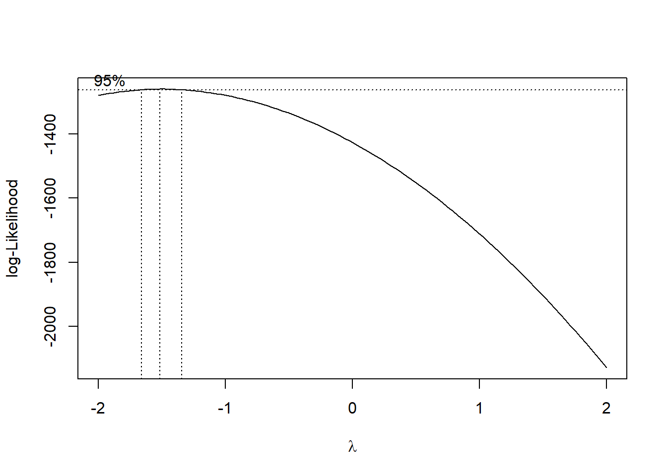
Figure 5.39: Box-Cox transformation: log-likelihood vs. lambda plot
The plot should have an upside-down U shape, and the optimal \(\lambda\) value is the one at which the log-likelihood is maximized. The object you assign the output to (below, bc) will contain elements \(x\) and \(y\) corresponding to the points being plotted to create the figure. These can be used to extract the optimal \(\lambda\) value using which().
## [1] -1.515The optimal value for this example is -1.515, which we can round to -1.5. Thus, our Box-Cox transformation is \((Y^{-1.5} - 1) / -1.5\). Interestingly, the optimal transformation turned out to be not that different from the inverse transformation (\(-Y^{-1}\)) that we earlier found in the small sample size version of this example to work better than a log or square root transformation.
Create the transformed version of the outcome and re-fit the model.
nhanesf.complete <- nhanesf.complete %>%
  mutate(LBDGLUSI_trans = (LBDGLUSI^LAMBDA - 1) / LAMBDA)

fit.ex5.1.trans <- lm(LBDGLUSI_trans ~ BMXWAIST + smoker +
    RIDAGEYR + RIAGENDR +  race_eth + income,
    data = nhanesf.complete)
NOTE: If the Box-Cox plot does not look like an upside down U, with a clear maximum, then increase the range over which to search \(\lambda\). For example, the following code tells the function to search over the range from –3 to 3.
Changing the range has the side effect of changing the resolution in the grid of possible values for \(\lambda\), but this difference will typically not matter, especially if you round to the nearest 0.1 afterwards. To increase the resolution of the grid, decrease the range and/or increase the length of the lambda argument in MASS::boxcox().
After using the Box-Cox outcome transformation, re-check the regression assumptions.
Re-check normality
Although the normality assumption is less important for this analysis due to the large sample size, for completeness we check it here. Previously, in Section 5.16, we checked this assumption for a model fit to a small subsample of the data; here, we will check the assumption for the model fit to the full dataset and the un-transformed outcome before re-checking it for the model with the transformed outcome.
The normality assumption remains violated (Figure 5.41) but much less so than before (Figure 5.40). However, the remaining violation is not an issue since the sample size is so large.
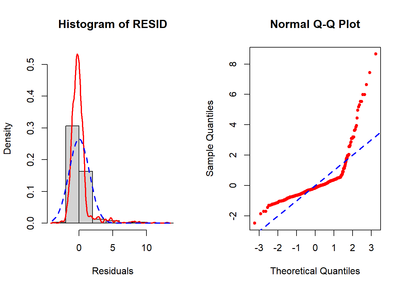
Figure 5.40: Check normality BEFORE using the Box-Cox transformation
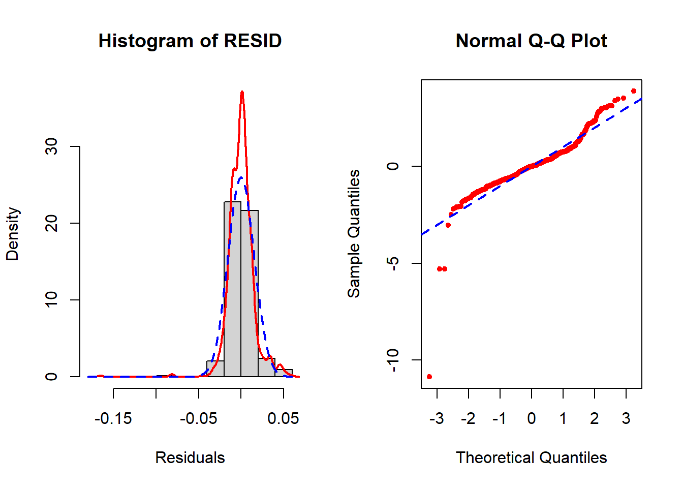
Figure 5.41: Re-check normality AFTER using the Box-Cox transformation
Re-check linearity
Before the outcome transformation, we resolved non-linearity using a quadratic transformation of waist circumference. However, after the Box-Cox outcome transformation, there is no non-linearity so no need for the quadratic transformation. It is generally safe to ignore minor non-linearities in areas of the plot with few points, such as on the far left of the CR plot for waist circumference (Figure 5.42).
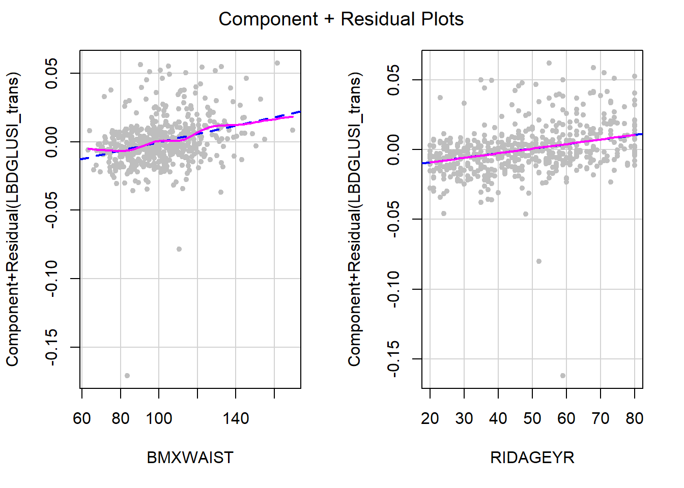
Figure 5.42: Re-check linearity after Box-Cox transformation
This illustrates that there may be multiple ways to resolve an assumption violation, and which you pick is more of an art than a science. In general, go with the solution that is simplest and easiest to explain. In this example, the outcome transformation is simpler than the quadratic predictor transformation in the sense that inference about the predictor’s relationship to the outcome involves just one regression coefficient instead of the two you would have with a quadratic transformation. On the other hand, the outcome transformation is more complicated in the sense that it leads to predictions that are not on the original outcome scale.
Re-check constant variance
The variance still seems to increase with the fitted values, but not as much as before we used the Box-Cox transformation. Additionally, there are a few points with large negative residuals (Figure 5.43). We will examine these outliers in Section 5.22.
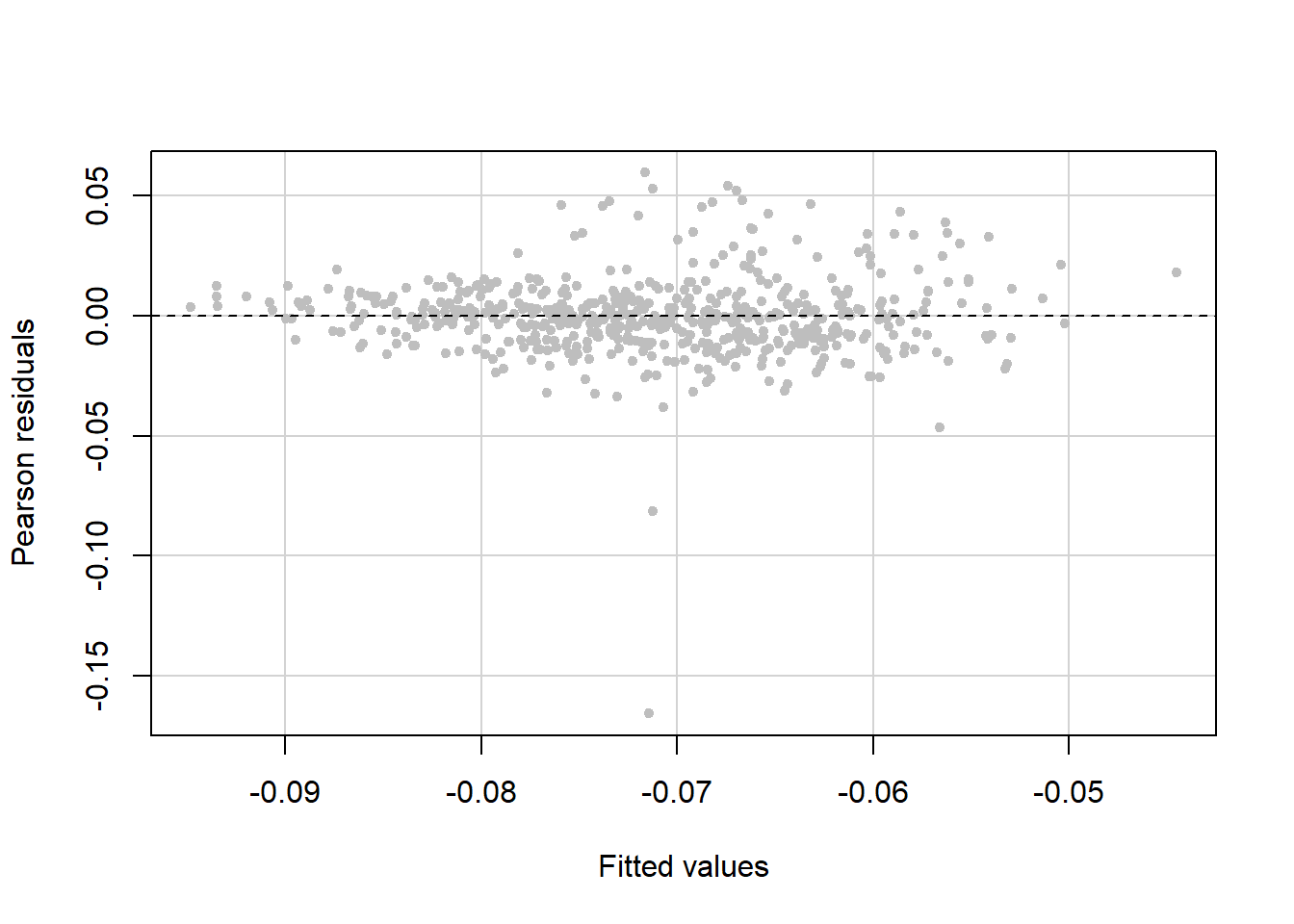
Figure 5.43: Re-check constant variance after Box-Cox transformation