9.4 Fitting the imputation model
Example 9.1: As an example, return to the linear regression of fasting glucose (mmol/L) (LBDGLUSI) on waist circumference (BMXWAIST) and smoking status (smoker; Never, Past, Current) in the NHANES 2017-2018 fasting subset teaching dataset (see Appendix A.1), adjusted for age (RIDAGEYR), gender (RIAGENDR; Male, Female), race/ethnicity (RIDRETH3; Mexican American, Other Hispanic, Non-Hispanic White, Non-Hispanic Black, Non-Hispanic Asian, Other/Multi), and income (<$25,000, $25,000 to <$55,000, $55,000+). Previously, in Chapter 5, a complete case analysis was carried out using listwise deletion. Now MI will be used to handle the missing data.
9.4.1 What variables to include
Include in the imputation model all variables that will be used in the analysis, including those with no missing values. The underlying principle is that the imputation model should be at least as complex as the analysis to be done later. Otherwise, information about the relationships between variables will be lost.
For example, if the analysis is a regression, then include the regression outcome and all the predictors in the same form they will be used in the regression model. This strategy is referred to as transform-then-impute (von Hippel 2009). Specifically, if any variable in the regression model is collapsed, transformed, or modified in any way, include the modified version in the imputation model instead of the original version. If a predictor has both linear and quadratic terms in the regression model, include both in the imputation model (see Section 9.6.3). If predictors are involved in an interaction in the regression model, make sure the imputation model reflects that interaction either via stratification or by explicitly including an interaction term in the imputation model (see Section 9.6.4).
Additionally, if there are auxiliary variables available, variables not in the regression model that are suspected to be related to the probability of missingness and/or to the values of incomplete variables in the imputation model, include them in the imputation model, as well.
Finally, do not impute values for variables that are impossible. For example, do not impute values for “age of first alcohol use” among those who have never used alcohol. Instead of imputing values for these individuals, exclude such individuals and recognize that the scope of the analysis would be “among those who have ever used alcohol”. An exception to excluding these individuals would be if “age of first alcohol use” is the time-to-event outcome in a survival analysis. In that case, prior to fitting the imputation model, set each missing value to that individual’s chronological age (or to missing if their chronological age is unknown) and the event indicator to 0 (to indicate censoring).
9.4.2 Transform-then-impute vs. impute-then-transform
If you need a variable transformation for the regression model, create it before carrying out multiple imputation and include it in the imputation model in that form. For example, if you need a Box-Cox outcome transformation (demonstrated in Section 9.4.3) or a quadratic term (demonstrated in Section 9.6.3), create the transformed variable or quadratic term and add it to the dataset before carrying out multiple imputation, not after.
This method is referred to as transform-then-impute and preserves the relationships between variables in the regression model, as opposed to impute-then-transform which can distort the relationships between variables. Transform-then-impute is the better method and leads to consistent results (von Hippel 2009).
9.4.3 Pre-processing
Prior to fitting the imputation model, do all the same data checking and cleaning steps you would for any regression analysis. For example, set missing value codes to NA, collapse sparse categorical variable levels, code categorical variables as factors, and compute any needed variable transformations.
NOTE: The methods in this chapter assume that the dataset contains only variables that are in the imputation model. Therefore, select() only those variables prior to fitting the imputation model.
Example 9.1 (continued): Imitate the pre-processing steps used when this analysis was done in Chapter 5. First, collapse the sparse race/ethnicity levels. Second, transform fasting glucose using the Box-Cox outcome transformation computed in Section 5.19, as that is the form of the outcome used in the analysis. Finally, select() just the variables to be included in the imputation model.
# Pre-processing
nhanes <- nhanes_adult_fast_sub %>%
    mutate(
      # (1) Collapse a sparse categorical variable
      race_eth = fct_collapse(RIDRETH3,
      "Hispanic" = c("Mexican American", "Other Hispanic"),
      "Non-Hispanic Other" = c("Non-Hispanic Asian", "Other/Multi")),
      # (2) Box-Cox transformation for our regression
      LBDGLUSI_trans = -1*LBDGLUSI^(-1.5)
      ) %>%
  # Select the variables to be included in the imputation model.
  # If any variables were modified, include only the modified version.
  # Exceptions (see Sections 9.6.3 and 9.6.4):
  #   If including a quadratic, also include the linear term.
  #   If including an interaction, also include the main effects.
  select(LBDGLUSI_trans, BMXWAIST, smoker, RIDAGEYR, RIAGENDR, race_eth, income)

# Shorten labels for race_eth so output fits on the page
levels(nhanes$race_eth) <- c("Hispanic", "NH White", "NH Black", "NH Other")
NOTES:
mice()by default checks for collinearity when fitting the imputation model. If a variable is perfectly collinear, it is removed and not imputed. If there is severe approximate collinearity, all variables are imputed, but highly collinear variables are removed from some of the chained models.- Some methods in this chapter will fail if a non-categorical variable is class
integer. You can check the class usingclass(dat$X)and ifintegeris returned, then convert to numeric usingmutate(X = as.numeric(X))during pre-processing.
9.4.4 Visualize the missing data pattern
Visualize the missing data pattern using md.pattern(), as shown in Figure 9.2. Each row is a block of cases with missing values on the same variables, the numbers on the left are the number of cases in each block, the numbers on the right are the number of variables with missing values in that block, and the numbers on the bottom are the number of cases with missing values for each variable individually. For example, 857 cases have no missing data, 15 cases have missing data on both waist circumference and income, the fourth block has two variables with missing values, and there are 123 cases with missing income.
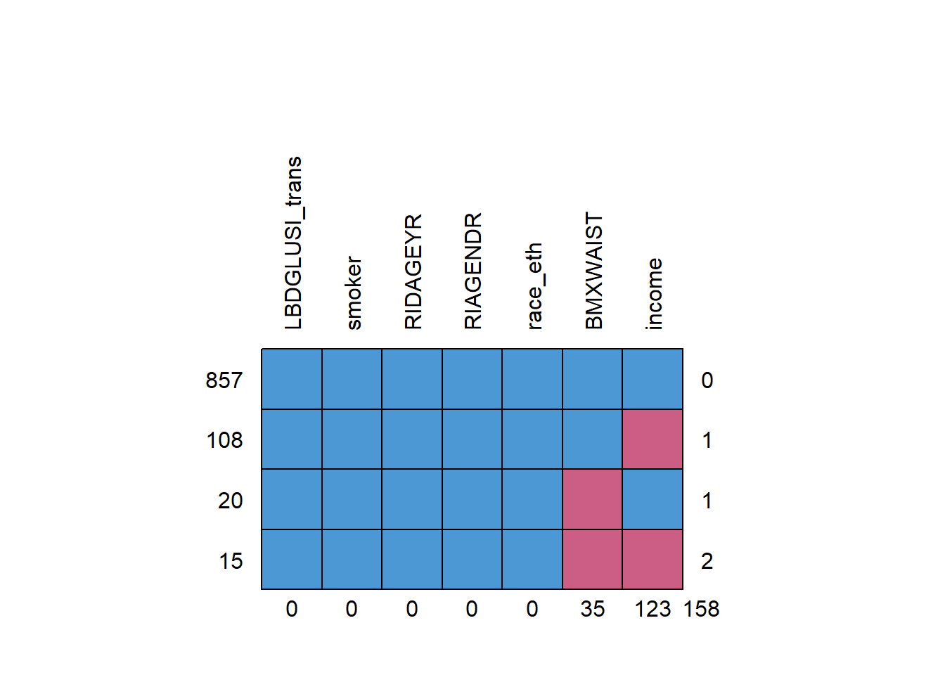
Figure 9.2: Missing data pattern
##     LBDGLUSI_trans smoker RIDAGEYR RIAGENDR race_eth BMXWAIST income
## 857              1      1        1        1        1        1      1   0
## 108              1      1        1        1        1        1      0   1
## 20               1      1        1        1        1        0      1   1
## 15               1      1        1        1        1        0      0   2
##                  0      0        0        0        0       35    123 158
NOTE: The number in the lower right (158) is the sum of the number of missing values across the variables. This is not necessarily the total number of incomplete cases, as some individuals may have a missing value for more than one variable. In this example, the number of incomplete cases is sum(!complete.cases(nhanes)) = 143, not 158.
9.4.5 Compare those with and without missing data
As mentioned previously, it is helpful for any research report to include a description of how the respondent characteristics differ between those with complete responses and those with item non-response. Split the sample once for each variable that has missing values and compare the other variables between each of the resulting pairs of samples.
If the distributions of the other variables are about the same in the complete and incomplete subgroups, that lends support to an assumption of MCAR and the use of a complete-case analysis. However, even if each other variable is similar between those with and without missing values for a variable, their joint distributions might not be similar. Additionally, if the number of cases with incomplete data is not small, a complete case analysis will result in lower precision due to the loss in sample size. Therefore, ultimately, this step of comparing those with and without missing data is not the basis for the decision regarding whether or not to use MI. If there is only a small fraction of missing values, a complete case analysis and MI will produce about the same results. If the fraction is larger, MI is superior whether the missing data mechanism is MCAR or not. This step is useful, however, as part of a complete description of the data and the nature of the missingness.
Example 9.1 (continued): For the NHANES teaching dataset, compare the descriptive statistics between those with and without missing data. This requires creating a missingness indicator for each variable with missing values to use as a “by” variable in the descriptive statistics table.
Look back at the visualization of missing data in the previous section, or use summary(), to see which variables have missing values in the dataset.
##  LBDGLUSI_trans       BMXWAIST         smoker       RIDAGEYR      RIAGENDR       race_eth
##  Min.   :-0.2372   Min.   : 63.2   Never  :579   Min.   :20.0   Male  :457   Hispanic:191
##  1st Qu.:-0.0813   1st Qu.: 88.3   Past   :264   1st Qu.:34.0   Female:543   NH White:602
##  Median :-0.0731   Median : 97.8   Current:157   Median :47.0                NH Black:115
##  Mean   :-0.0715   Mean   :100.5                 Mean   :47.9                NH Other: 92
##  3rd Qu.:-0.0645   3rd Qu.:111.0                 3rd Qu.:61.0
##  Max.   :-0.0121   Max.   :169.5                 Max.   :80.0
##                    NA's   :35
##                  income
##  <$25,000           :164
##  $25,000 to <$55,000:224
##  $55,000+           :489
##  NA's               :123
##
##
##
Since there are only two variables with missing values, we can create two tables and merge them together. If there were more than a few variables with missing values, such a merged table might be too large, in which case just look at each table individually.
NOTE: Below, missing is created only for the purpose of creating the table. Do not permanently add missing to the dataset, as that variable should not be included in the imputation model later.
The results are shown in Table 9.1.
library(gtsummary)
t1 <- nhanes %>%
  mutate(missing = factor(is.na(BMXWAIST),
                          levels = c(FALSE, TRUE),
                          labels = c("Not Missing",
                                     "Missing"))) %>%
  tbl_summary(
    by = missing,
    statistic = list(all_continuous()  ~ "{mean} ({sd})",
                     all_categorical() ~ "{n}    ({p}%)"),
    digits = list(all_continuous()  ~ c(2, 2),
                  LBDGLUSI_trans    ~ c(4, 4),
                  all_categorical() ~ c(0, 1)),
    label = list(LBDGLUSI_trans ~ "Transformed FG",
                 BMXWAIST ~ "WC (cm)",
                 smoker ~ "Smoking",
                 RIDAGEYR ~ "Age (y)",
                 RIAGENDR ~ "Gender",
                 race_eth ~ "Race/Ethnicity",
                 income ~ "Income")
  ) %>%
  modify_header(
    label = "**Variable**",
    all_stat_cols() ~ "**{level}**<br>N = {n} ({style_percent(p, digits=1)}%)"
  ) %>%
  modify_caption("Participant characteristics, by missingness") %>%
  bold_labels()

t2 <- nhanes %>%
  mutate(missing = factor(is.na(income),
                          levels = c(FALSE, TRUE),
                          labels = c("Not Missing",
                                     "Missing"))) %>%
  tbl_summary(
    by = missing,
    statistic = list(all_continuous()  ~ "{mean} ({sd})",
                     all_categorical() ~ "{n}    ({p}%)"),
    digits = list(all_continuous()  ~ c(2, 2),
                  LBDGLUSI_trans    ~ c(4, 4),
                  all_categorical() ~ c(0, 1)),
    label = list(LBDGLUSI_trans ~ "Transformed FG",
                 BMXWAIST ~ "WC (cm)",
                 smoker ~ "Smoking",
                 RIDAGEYR ~ "Age (y)",
                 RIAGENDR ~ "Gender",
                 race_eth ~ "Race/Ethnicity",
                 income ~ "Income")
  ) %>%
  modify_header(
    label = "**Variable**",
    all_stat_cols() ~ "**{level}**<br>N = {n} ({style_percent(p, digits=1)}%)"
  )

TABLE <- tbl_merge(
  tbls = list(t1, t2),
  tab_spanner = c("**Waist Circumference**", "**Income**")
)| Variable |
Waist Circumference
|
Income
|
||
|---|---|---|---|---|
| Not Missing N = 965 (96.5%)1 |
Missing N = 35 (3.50%)1 |
Not Missing N = 877 (87.7%)1 |
Missing N = 123 (12.3%)1 |
|
| Transformed FG | -0.0715 (0.0173) | -0.0734 (0.0174) | -0.0714 (0.0176) | -0.0727 (0.0148) |
| WC (cm) | 100.48 (16.95) | NA (NA) | 100.82 (17.15) | 97.73 (15.03) |
| Unknown | 0 | 35 | 20 | 15 |
| Smoking | ||||
| Never | 557 (57.7%) | 22 (62.9%) | 511 (58.3%) | 68 (55.3%) |
| Past | 255 (26.4%) | 9 (25.7%) | 228 (26.0%) | 36 (29.3%) |
| Current | 153 (15.9%) | 4 (11.4%) | 138 (15.7%) | 19 (15.4%) |
| Age (y) | 47.70 (16.46) | 52.63 (20.90) | 47.84 (16.55) | 48.12 (17.41) |
| Gender | ||||
| Male | 443 (45.9%) | 14 (40.0%) | 398 (45.4%) | 59 (48.0%) |
| Female | 522 (54.1%) | 21 (60.0%) | 479 (54.6%) | 64 (52.0%) |
| Race/Ethnicity | ||||
| Hispanic | 180 (18.7%) | 11 (31.4%) | 157 (17.9%) | 34 (27.6%) |
| NH White | 589 (61.0%) | 13 (37.1%) | 544 (62.0%) | 58 (47.2%) |
| NH Black | 111 (11.5%) | 4 (11.4%) | 100 (11.4%) | 15 (12.2%) |
| NH Other | 85 (8.8%) | 7 (20.0%) | 76 (8.7%) | 16 (13.0%) |
| Income | ||||
| <$25,000 | 157 (18.3%) | 7 (35.0%) | 164 (18.7%) | 0 (NA%) |
| $25,000 to <$55,000 | 221 (25.8%) | 3 (15.0%) | 224 (25.5%) | 0 (NA%) |
| $55,000+ | 479 (55.9%) | 10 (50.0%) | 489 (55.8%) | 0 (NA%) |
| Unknown | 108 | 15 | 0 | 123 |
| 1 Mean (SD); n (%) | ||||
Summary:
- Those with missing waist circumference have, on average, lower fasting glucose and older age, are less likely to smoke, and are more likely to be female, Hispanic or non-Hispanic Other race, and earn <$25,000 per year.
- Those with missing income have, on average, lower fasting glucose and smaller waist circumference, and are more likely to be Hispanic or non-Hispanic Other race.
9.4.6 Number of imputations
If you need to try out different options in the mice() function, then use a small number of imputations (e.g., 5), as that will speed up processing while you work out the details of your code. When you are ready to fit your final imputation model, however, use 20 imputations. That is actually the first step in the method of von Hippel (2020). However, it is easier to learn other aspects of multiple imputation first, so the details of that method will be left to Section 9.9.
9.4.7 mice()
Use the mice() function to fit the imputation model. Since MI involves random draws from distributions, each time you run mice() you will get slightly different results. To ensure reproducibility, use the seed option to set the random seed to any number you choose (use seed = 3 to reproduce the results in this text). The m option specifies the number of imputations, and print = F suppresses a listing of the iterations. The first argument to the function is the dataset containing only the variables to be included in the imputation model; any variable that is not part of the imputation model should be excluded from this dataset.
Example 9.1 (continued): Fit the imputation model and examine the output.
## Class: mids
## Number of multiple imputations:  20
## Imputation methods:
## LBDGLUSI_trans       BMXWAIST         smoker       RIDAGEYR       RIAGENDR       race_eth
##             ""          "pmm"             ""             ""             ""             ""
##         income
##      "polyreg"
## PredictorMatrix:
##                LBDGLUSI_trans BMXWAIST smoker RIDAGEYR RIAGENDR race_eth income
## LBDGLUSI_trans              0        1      1        1        1        1      1
## BMXWAIST                    1        0      1        1        1        1      1
## smoker                      1        1      0        1        1        1      1
## RIDAGEYR                    1        1      1        0        1        1      1
## RIAGENDR                    1        1      1        1        0        1      1
## race_eth                    1        1      1        1        1        0      1
The output states that the object named imp.nhanes is of class mids (multiply imputed dataset), the number of imputations (20), the Imputation method used for each variable, and which variables were used to predict which other variables (PredictorMatrix). By default, mice() used predictive mean matching (pmm) for waist circumference (a continuous variable) and multinomial logistic regression (polyreg) for income (less restrictive than using ordinal logistic regression). The PredictorMatrix will generally have 0s on the diagonal and 1s elsewhere indicating that each variable is predicted using all the others.
Some methods used later in this chapter operate directly on a mids object, but others require first extracting the individual imputed datasets. complete() converts a mids object to either a single complete dataset or all the completed datasets. There are a number of different ways of doing this. The two used in this chapter are returning the first imputed dataset and returning the original data and all imputed datasets all in one stacked dataset.
# Return the first imputed dataset
imp.nhanes.dat <- complete(imp.nhanes)
# Same dimensions as original data
dim(nhanes)
## [1] 1000 7## [1] 1000 7# Return all the imputed datasets in "long" form (they will be stacked vertically)
# including the original (unimputed) data
imp.nhanes.dat <- complete(imp.nhanes, "long", include = TRUE)
# imp.nhanes$m*(n+1) rows
dim(imp.nhanes.dat)## [1] 21000 9## [1] "LBDGLUSI_trans" "BMXWAIST" "smoker" "RIDAGEYR" "RIAGENDR"
## [6] "race_eth" "income" ".imp" ".id"# A new variable called ".imp" is created that indexes the imputations
# .imp = 0 corresponds to the original data
# .imp = 1 to m corresponds to the imputed data
range(imp.nhanes.dat$.imp) # 0 to m## [1] 0 20# A new variable called ".id" is created that indexes the observations
range(imp.nhanes.dat$.id) # 1 to number of cases## [1] "100" "999"9.4.8 Examine the imputed values
After fitting the imputation model, examine the imputations by plotting the observed and imputed data together. Ideally, the imputed values are plausible compared to the observed values. Imputed values that are far away from the distribution of the observed values (not possible with pmm but possible with other methods) may indicate a problem with the imputation model, or perhaps that an MNAR model is needed. Imputed values which only span a subset of the distribution of the observed values are interesting in that they provide some information about the nature of the missing values that may assist in reducing missing data in future studies.
stripplot() plots the observed and missing values for continuous variables (Figure 9.3). The observed data are plotted (labeled as 1 on the x-axis) as well as the observed and imputed data together for each completed dataset (labeled as 2 to the number of imputations + 1 on the x-axis). The points are “jittered” to provide some spread, so it is easier to see the imputed values superimposed over the observed values. By default, stripplot() will make plots even for variables with no missing data, but a formula can be included to specify just a variable with missing data (in our example, BMXWAIST ~ .imp, where .imp is a special variable referring to the imputation number). The col, pch, and cex options specify the color, plotting character, and point size, respectively. For each, specify two values, the first for the observed values, the second for the imputed values.
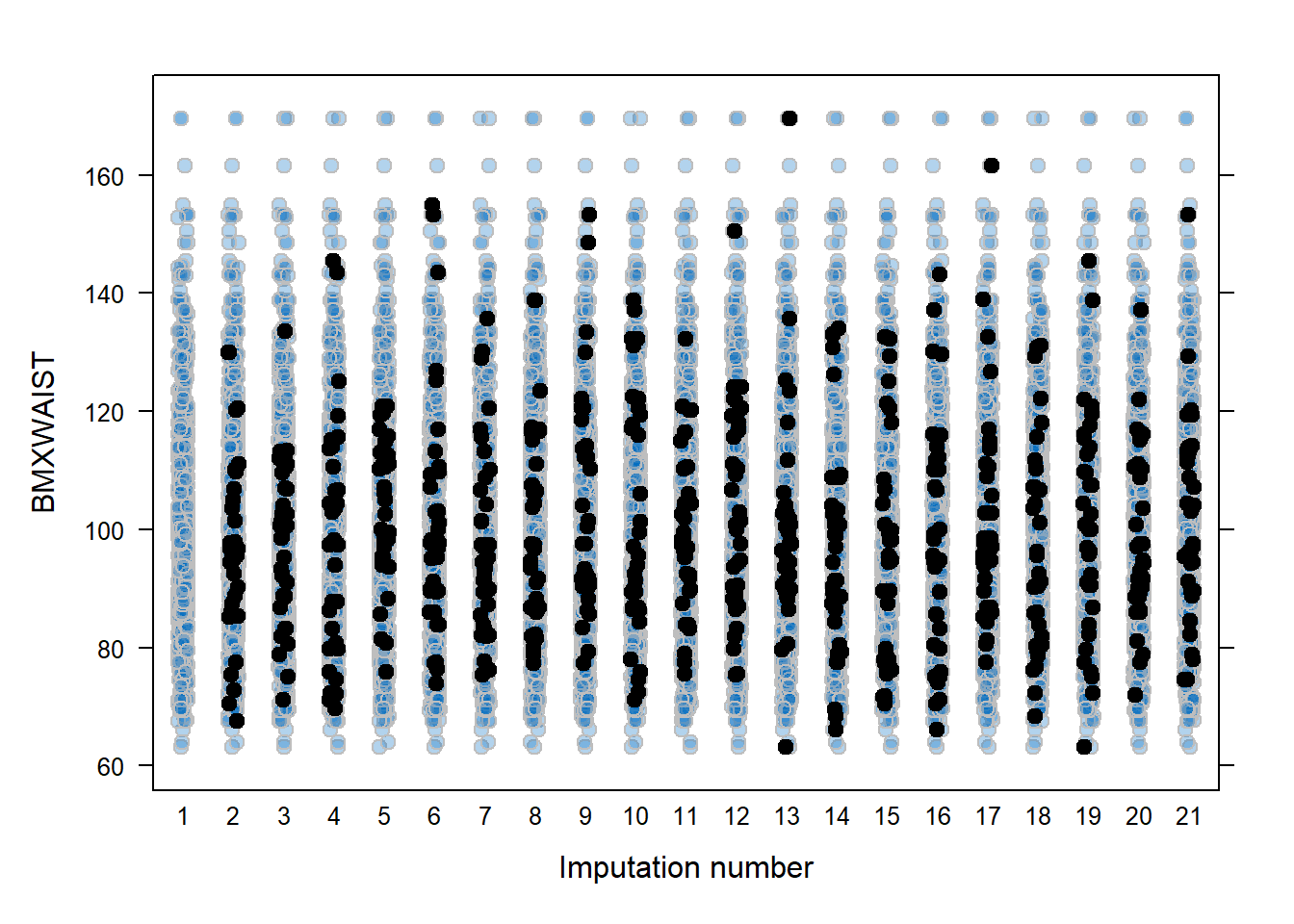
Figure 9.3: All observed and imputed values, by imputation
Alternatively, you can plot the imputed values by another variable.
# vs. a categorical variable (results not shown)
stripplot(imp.nhanes, BMXWAIST ~ RIAGENDR,
          col = c("gray", "black"),
          pch = c(21, 20),
          cex = c(1, 1.5))

# vs. a continuous variable (results not shown)
stripplot(imp.nhanes, BMXWAIST ~ LBDGLUSI_trans,
          col = c("gray", "black"),
          pch = c(21, 20),
          cex = c(1, 1.5))
If the number of missing values is large, stripplot() might not be very informative since imputed values are plotted on top of observed values. An alternative is to use bwplot() to plot side-by-side boxplots (Figure 9.4). With this function, the observed data are labeled as imputation 0 on the x-axis, and the boxplots for each imputation only plot the distribution of imputed values.
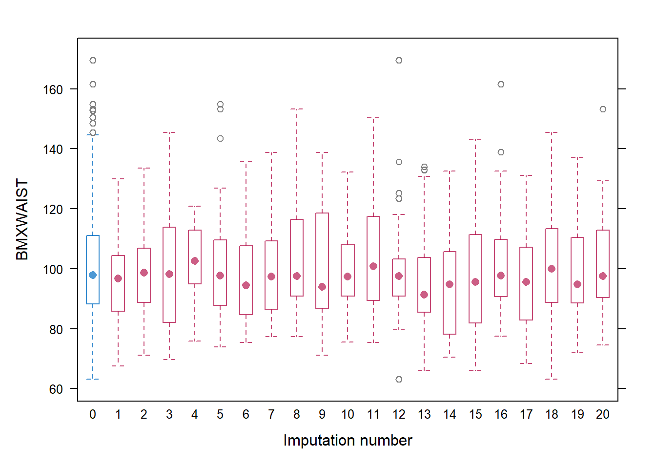
Figure 9.4: Boxplots of observed and imputed values, by imputation
For a categorical variable, create a two-way table comparing the distribution of the variable between the complete data and the imputed data. This requires using the “long” form of the data, including the original data.
imp.nhanes.dat <- complete(imp.nhanes, "long", include = TRUE)

imp.nhanes.dat <- imp.nhanes.dat %>%
  mutate(imputed = .imp > 0,
         imputed = factor(imputed,
                          levels = c(F,T),
                          labels = c("Observed", "Imputed")))

prop.table(table(imp.nhanes.dat$income,
                 imp.nhanes.dat$imputed),
           margin = 2)
##
## Observed Imputed
## <$25,000 0.1870 0.1889
## $25,000 to <$55,000 0.2554 0.2584
## $55,000+ 0.5576 0.5527The following code creates a table that includes a separate column for each imputation.
9.4.9 For descriptive statistics only: back-transformation and derived variables
If there are variables you transformed for the imputation and regression models, but want to include on their original scale for descriptive statistics, then you must back-transform them after imputation. Similarly, if there are new variables, not in the imputation model, that you would like to derive based on the variables in the imputation model, derive them after imputation and add them to the imputed datasets; however, it is critical that you do not include the post-imputation back-transformed or derived variables in the regression model; they are only to be used for descriptive statistics.
Very important: To re-iterate, back-transformation is not to be used to derive variables for inclusion in a regression model; doing so would be impute-then-transform which results in a distortion of the relationship between the variables in the regression model (as described in Section 9.4.2). If you need a variable for the regression model, create it in the pre-processing step and include it in the imputation model in that form (Section 9.4.3). Back-transformation is only to be used to un-transform or derive variables for the purpose of descriptive statistics, not for inclusion in the regression model.
Example 9.1 (continued): For fasting glucose, we need the transformed variable for the regression model. However, we would like the original variable for computing descriptive statistics. Additionally, we would like to compute descriptive statistics by waist circumference, but since it is a continuous variable we need to derive a median split version for use as our “by” variable.
The code below demonstrates how to back-transform a variable, create a derived variable, and include these in the imputed datasets. First, extract the imputed datasets in “long” form from the mids object. Second, manipulate the long-form dataset (e.g., using a mutate() statement). Finally, convert the long-form dataset back into a mids object.
# Use complete() to extract all the imputed datasets, with
# include = TRUE to also extract the original incomplete dataset
imp.nhanes.dat <- complete(imp.nhanes, "long", include = TRUE)

# Inverse Box-Cox transformation
# If Z = -1*Y^(-1.5),  then Y = (-Z)^(1/-1.5)
imp.nhanes.dat <- imp.nhanes.dat %>%
  mutate(LBDGLUSI = (-1*LBDGLUSI_trans)^(1/-1.5))

# Median split
MEDIAN <- median(imp.nhanes.dat$BMXWAIST, na.rm = T)
LABEL0 <- paste("WC <",  MEDIAN, sep = "")
LABEL1 <- paste("WC >=", MEDIAN, sep = "")

imp.nhanes.dat <- imp.nhanes.dat %>%
  mutate(wc_median_split = as.numeric(BMXWAIST >= MEDIAN),
         wc_median_split = factor(wc_median_split,
                                  levels = 0:1,
                                  labels = c(LABEL0, LABEL1)))

# Convert back to a `mids` object
imp.nhanes.new <- as.mids(imp.nhanes.dat)
As always, do a before vs. after check to make sure any back-transformations or derivations did what you expected. In particular, make sure the back-transformed variable is on the same scale as the corresponding original variable, but do not be concerned if the summary() before vs. after is not exactly identical since any previously missing values are now imputed. This check is especially important when back-transforming a Box-Cox transformed variable, as it is easy to put a parenthesis in the wrong place resulting in the wrong formula.
##    Min. 1st Qu.  Median    Mean 3rd Qu.    Max.
## 2.61 5.33 5.72 6.09 6.22 19.00## Min. 1st Qu. Median Mean 3rd Qu. Max.
## 2.61 5.33 5.72 6.09 6.22 19.00# Check derivation of median split
tapply(imp.nhanes.dat$BMXWAIST,
imp.nhanes.dat$wc_median_split, range)## $`WC <97.8`
## [1] 63.2 97.7
##
## $`WC >=97.8`
## [1] 97.8 169.5