9.8 Cox regression after MI
MI with time-to-event data that includes censoring is more complex than what we have seen so far. The issue is that the outcome is not just a single variable, but a pair of variables, the event time and the event indicator, with the event time being censored for those with event indicator = 0. The obvious solution is to include both the event indicator and time in the imputation model. However, a better approach is to include in the imputation model the event indicator and, instead of the event time, the cumulative baseline hazard, and possibly also the interaction between the event indicator and the cumulative baseline hazard (I. R. White and Royston 2009). The hazard function was discussed in Section 7.4. The baseline hazard is the hazard function when all predictors are at zero or their reference level, and the cumulative baseline hazard sums the baseline hazard up to a given time.
The strategy is to compute each individual’s cumulative baseline hazard at their event time using the mice function nelsonaalen() and add it to the dataset in place of the event time, carry out MI using mice(), and put the event time back into the imputed datasets before fitting the Cox model on each imputed dataset and pooling the results.
Example 9.3: Using the Natality teaching dataset (see Appendix A.3), estimate the association between previous preterm birth (RF_PPTERM) and time to preterm birth, adjusted for mother’s age (MAGER), race/ethnicity (MRACEHISP), and marital status (DMAR). The event time and event indicator variables are gestage37 and preterm01, respectively. Handle missing data using MI.
load("Data/natality2018_rmph.Rdata")

# Compute cumulative baseline hazard and add to the dataset
natality$cumhaz <- nelsonaalen(natality, gestage37, preterm01)
What is this actually doing? Each individual has an event time. We could include that time in the imputation model. Doing so would mean that we think the predictors are associated linearly with the event time. What makes more sense, however, is to assume that the predictors are associated with the risk of the event at a given time. It turns out that the appropriate term to put into the imputation model is the cumulative baseline hazard up to that time. This replaces linear time with a non-linear function of time. In Figure 9.6, we see that below about 26 weeks the cumulative baseline hazard is relatively constant, and then increases non-linearly. Using linear time in the imputation model would be equivalent to assuming the accumulation of risk is constant over time, which is generally not realistic.
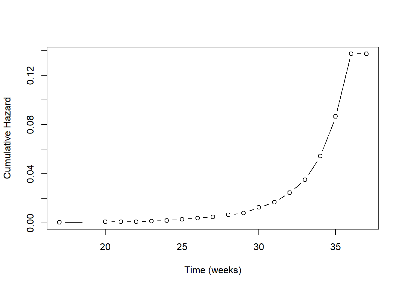
Figure 9.6: Cumulative baseline hazard vs. time
Next, fit the imputation model, including cumhaz instead of the time variable.
# Select the variables for inclusion in the imputation model
# Include the cumulative baseline hazard
# Include the event indicator variable
# Do NOT include the event time variable
natality_for_imp <- natality %>%
  select(cumhaz, preterm01, RF_PPTERM, MAGER, MRACEHISP, DMAR)

imp.natality <- mice(natality_for_imp,
                     seed  = 3,
                     m     = 20,
                     print = F)
Next, put the time variable back into the dataset for use in coxph(). If there were any missing time values, replace them with imputed values. This is done by creating a look-up table (bhz) and finding the time value that corresponds to each imputed cumhaz value. This works because the baseline cumulative hazard depends only on time, not on any of the predictors in the model.
NOTE: The code below only works if predictive mean matching (the default) was used to impute missing cumulative baseline hazard values.
# Imputed datasets in long form
imp.natality.dat <- complete(imp.natality, "long", include = TRUE)

# Repeat time variable m + 1 times since impdat
# includes the original data as well as m imputations
imp.natality.dat$gestage37 <- rep(natality$gestage37, imp.natality$m + 1)

# Replace missing time values with time corresponding
# to the imputed cumulative hazard value
# (only needed if there were missing event times,
#  but no harm in running if there were not)
#  .imp > 0 prevents replacing missing values in the original data
SUB <- imp.natality.dat$.imp > 0 & is.na(imp.natality.dat$gestage37)
if(sum(SUB) > 0) {
  # Create a look-up table with the event times
  # and corresponding cumulative hazards
  bhz <- data.frame(time   = natality$gestage37,
                    cumhaz = natality$cumhaz)
  # Sort and remove duplicates
  bhz <- bhz[order(bhz$time),]
  bhz <- bhz[!duplicated(bhz) & complete.cases(bhz$time),]

  # The following only works if pmm (the default) was used
  # to impute missing cumhaz values
  # (because it relies on the imputed values being values
  #  present in the non-missing values)
  for(i in 1:sum(SUB)) {
    # Use max since last 2 times have the same cumhaz
    imp.natality.dat$gestage37[SUB][i] <-
      max(bhz$time[bhz$cumhaz == imp.natality.dat$cumhaz[SUB][i]], na.rm = T)
  }
}

# Convert back to a mids object
imp.natality.new <- as.mids(imp.natality.dat)
Finally, fit the Cox regression on the imputed datasets and display the pooled results.
NOTE: Only include in the regression model variables that were included in the dataset prior to multiple imputation (see Section 9.4.2).
library(survival)
fit.imp.cox <- with(imp.natality.new,
                coxph(Surv(gestage37, preterm01) ~
                      RF_PPTERM + MAGER + MRACEHISP + DMAR))
# Do NOT include the -1 here since a Cox model has no intercept
# summary(pool(fit.imp.cox), conf.int = T,
#         exponentiate = T)[, c("term", "estimate", "2.5 %", "97.5 %", "p.value")]
round.summary(fit.imp.cox, digits = 3,
              exponentiate = T)[, c("estimate", "2.5 %", "97.5 %", "p.value")]
## estimate 2.5 % 97.5 % p.value
## RF_PPTERMYes 3.213 2.079 4.966 0.000
## MAGER 1.031 1.008 1.054 0.007
## MRACEHISPNH Black 1.858 1.322 2.613 0.000
## MRACEHISPNH Other 1.111 0.685 1.801 0.668
## MRACEHISPHispanic 1.328 0.965 1.828 0.082
## DMARUnmarried 1.822 1.339 2.479 0.000