4.1 Introduction

In general, a regression analysis estimates the association between an outcome \((Y)\) and one or more predictors \((X_1,X_2,…,X_K)\). Linear regression is used when \(Y\) is continuous. The term simple linear regression (SLR) is typically used for the setting where there is only one predictor \((X)\) and that predictor is continuous. In this text, the term SLR refers to any linear regression with just one predictor, whether that predictor is continuous, categorical, or modeled as a curve (e.g., a quadratic polynomial). Chapter 5 extends SLR to the case of multiple predictors (multiple linear regression, MLR). This chapter is not meant to be an exhaustive treatment of SLR. Rather, it is meant to give just enough of an introduction to the concepts of linear regression to set the stage for MLR.

Two examples are used throughout this chapter to demonstrate the use of R for SLR. The remainder of this introduction presents some basic analyses to set the stage, along with some example R code for visualizing the relationship between the outcome and predictor.

Example 4.1: Levels of fasting glucose, measured using a blood draw following a fast, are one criteria used to diagnose Type 2 diabetes. An individual is classified as “normal”, “pre-diabetic”, or “diabetic” if their fasting glucose is <5.6 mmol/L, 5.6–6.9 mmol/L, or 7 mmol/L or greater on two separate tests, respectively (https://www.mayoclinic.org/diseases-conditions/type-2-diabetes/diagnosis-treatment/drc-20351199, Accessed September 17, 2021). The code below investigates the distribution of fasting glucose (mmol/L) using data from adults age \(\ge\) 20 years in NHANES 2017-2018. The teaching dataset nhanes1718_adult_fast_sub_rmph.Rdata contains a random subsample of 1,000 adults who had blood drawn after fasting (see Appendix A.1). After investigating the distribution, investigate how the mean fasting glucose varies with waist circumference (a continuous predictor).

After loading the data, use a histogram to examine the distribution of fasting glucose (LBDGLUSI) and add a vertical line to visualize the location of the average value (Figure 4.1).

load("Data/nhanes1718_adult_fast_sub_rmph.Rdata")
# For convenience, give the dataset a shorter name
nhanesf <- nhanes_adult_fast_sub

hist(nhanesf$LBDGLUSI, xlab = "Fasting Glucose (mmol/L)", main =  "", breaks = 20)
MEAN <- mean(nhanesf$LBDGLUSI, na.rm = T)
abline(v = MEAN, lwd = 3, col = "red")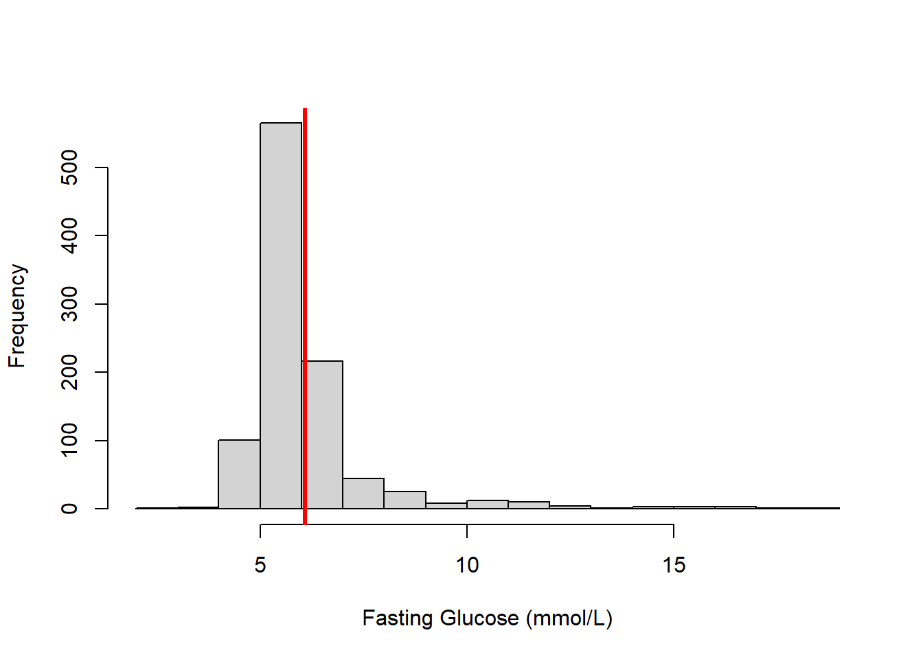

Figure 4.1: Histogram of fasting glucose (vertical bar indicates the mean value)

The notation \(E(Y)\) refers to the “expected value” or mean of a random variable \(Y\). In this sample, the average fasting glucose (FG) is 6.1 mmol/L; thus, \(E(FG)\) = 6.1. This is the average value, but the histogram demonstrates that there is a lot of variation between individuals. Is there some other variable that might explain some of that variation? We might hypothesize that groups of people with different amounts of body fat have different average values of fasting glucose.

Below, we examine how fasting glucose is associated with body fat, using waist circumference (BMXWAIST) as our measure of adiposity. If you are only interested in a measure of association, then estimating the correlation would be enough, and we could compute that the correlation between fasting glucose and waist circumference is .295.

cor(nhanesf$LBDGLUSI, nhanesf$BMXWAIST, use = "complete.obs")

## [1] 0.2952

But SLR can do more than just estimate a measure of association; it can find the best fitting line describing the linear relationship between fasting glucose and waist circumference, as shown in Figure 4.2.

plot(LBDGLUSI ~ BMXWAIST, data = nhanesf,
     col = "gray",
     ylab = "Fasting Glucose (mmol/L)",
     xlab = "Waist Circumference (cm)",
     las = 1,  # Rotate the axis labels so they are all horizontal
     pch = 20, # Change the plotting symbol to solid circles 
     font.lab = 2, font.axis = 2) # Bold font
# The lm() function fits a linear regression (discussed more later)
abline(lm(LBDGLUSI ~ BMXWAIST, data = nhanesf), lwd = 2, col = "red")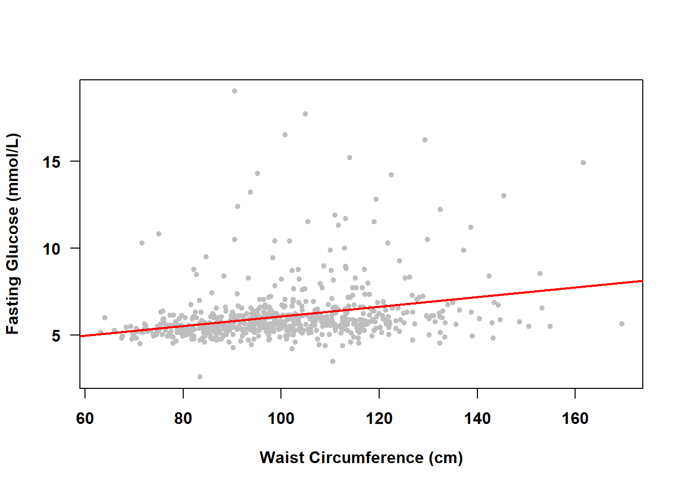

Figure 4.2: Simple linear regression of fasting glucose on waist circumference

With just the mean all we had was \(E(FG)\); now we have \(E(FG|WC)\), which is read as “the expected value of fasting glucose given waist circumference”. The line in Figure 4.2 shows us how fasting glucose differs, on average, between individuals with different waist circumference, which is much more informative than just the single, overall, mean value.

In Example 4.1, the predictor variable is continuous. When the predictor is categorical, taking on only a few values, then rather than fit a straight line SLR estimates the mean outcome at each discrete level of the predictor.

Example 4.2: How does average fasting glucose differ between never, past, and current smokers (smoker)?

# NOTE: plot.default is used because plot results in boxplots
#       instead of the actual data points.
#       plot.default does not have a data argument so we must
#       extract y and x using the $ notation.
plot.default(nhanesf$LBDGLUSI ~ nhanesf$smoker,
             col = "gray",
             ylab = "Fasting Glucose (mmol/L)",
             xlab = "Smoking Status", 
             las = 1, pch = 20, font.lab = 2, font.axis = 2,
             xaxt = "n") # Suppresses the x-axis
# Add custom x-axis
axis(1, at = 1:3, labels = levels(nhanesf$smoker), font = 2)
# Compute means
MEANS <- tapply(nhanesf$LBDGLUSI, nhanesf$smoker, mean, na.rm = T)
# Add means to the plot
# NOTE: For points() and lines() the arguments are x, y not y ~ x
points(1:3, MEANS, pch = 20, cex = 3)
lines( 1:3, MEANS, col = "red", lwd=2)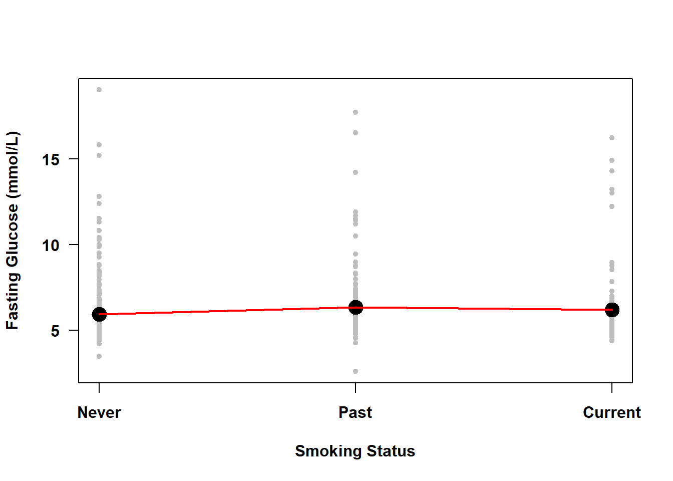

Figure 4.3: Simple linear regression of fasting glucose on smoking status

The line connecting the mean fasting glucose at different levels of smoking status in Figure 4.3 is not estimated by SLR; it is just added here to demonstrate that with a categorical predictor the means are not constrained to fall on a straight line.

NOTE: This is not a book about R programming, but rather how to use R to do regression analyses. If you are still relatively new to R and want to learn more about how a code chunk presented in this text works, then play around with changing different options or investigating pieces of the code. For example, change the value of font.lab in the previous code chunk and see what changes in the plot; or type MEANS in the R console to see what output tapply() produces; or type ?tapply to learn more about that function.