2.1 Introduction

Introductory statistics classes often cover methods for testing and assessing the magnitude of an association between two variables, such as correlation, the two-sample t-test, analysis of variance, the chi-square test, and others. Regression is a general term used for methods that assess the association between an outcome and one or more predictors by positing a model for the outcome as a function of the predictors. Many basic statistical methods are actually special cases of regression with a single predictor.

Unlike, for example, correlation, in regression you must designate one variable to be the outcome, also known as the dependent variable. The other variables are predictors, or independent variables. In some contexts, predictors may be referred to as covariates or confounders.

A simple linear regression model has the following equation.

\[\begin{equation} Y = \beta_0 + \beta_1 X + \epsilon \tag{2.1} \end{equation}\]

Chapter 4 will explain what all these symbols represent, but for now just know that Equation (2.1) describes a model in which the values of an outcome \(Y\) are linearly related to the values of a predictor \(X\) – pairs of points \((X,Y)\) are scattered randomly around a line. Figure 2.1 illustrates data generated from a simple linear regression model. At each \(X\) value, the corresponding \(Y\) value is the sum of the height of the line at \(X\) and some random noise.

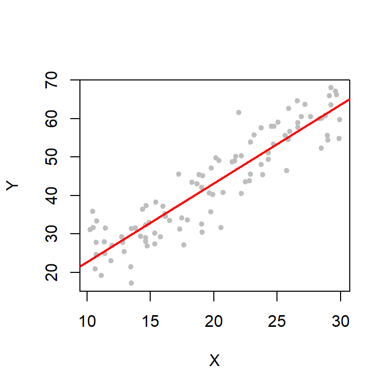
Figure 2.1: Linear regression example

In practice, \(Y\) is some outcome of interest (e.g., fasting glucose) and \(X\) is candidate predictor of that outcome (e.g., body fat). If the line has a positive slope (as in Figure 2.1), we say that the predictor has a positive association with the outcome – individuals with larger \(X\) values tend to have larger \(Y\) values. If the line has a negative slope, the opposite would be true – individuals with larger \(X\) values tend to have smaller \(Y\) values.

More complicated regression settings have equations that are more complicated than Equation (2.1), including perhaps having more than one predictor. For example, a multiple linear regression model with \(K\) predictors is described by Equation (2.2).

\[\begin{equation} Y = \beta_0 + \beta_1 X_1 + \beta_2 X_2 + \ldots + \beta_K X_K + \epsilon \tag{2.2} \end{equation}\]