5.10 Interactions
In the MLR models we have encountered so far, each regression coefficient is interpreted as the effect of a predictor while holding other predictors at fixed values and the effect does not depend on at which specific values you hold the other predictors. How do we model a scenario in which the effect does depend on the level of one of the other variables? This is accomplished by including an interaction in the model and treats the other variable as a moderator (effect modifier) (Section 5.9). An interaction between two predictors is referred to as a two-way interaction. It is possible to have three-way (or more way) interactions, but this section will only discuss two-way interactions.
5.10.1 Understanding a two-way interaction using stratification
Effect modification and the use of interactions tend to be challenging for many students of regression when first encountered. Rather than diving straight into the details of including an interaction in a regression model, we start by clarifying what an interaction is through the use of stratification. As described at the end of Section 5.9.3, including an interaction is similar to stratifying the analysis by another variable and estimating the effect of a variable within levels of another.
Example 5.2: In the regression of fasting glucose on waist circumference, does the effect of waist circumference on fasting glucose depend on gender? Stratify by gender, fit a regression model for each gender, and compare the waist circumference effects between the two models. Are they the same or different? If they are different, then gender is an effect modifier (it modifies the waist circumference association with fasting glucose).
# Stratify by gender
nhanesf.complete.M <- nhanesf.complete %>%
  filter(RIAGENDR == "Male")
nhanesf.complete.F <- nhanesf.complete %>%
  filter(RIAGENDR == "Female")
Run the following to verify that the code results in datasets of the correct size.
# Check
table(nhanesf.complete$RIAGENDR, useNA = "ifany")
nrow(nhanesf.complete.M)
nrow(nhanesf.complete.F)
# Fit for Males
fit.ex5.2.strat.M <- lm(LBDGLUSI ~ BMXWAIST, data = nhanesf.complete.M)
# Fit for Females
fit.ex5.2.strat.F <- lm(LBDGLUSI ~ BMXWAIST, data = nhanesf.complete.F)
# Fit ignoring gender (for comparison)
# (fit earlier)
# fit.ex4.1.cc <- lm(LBDGLUSI ~ BMXWAIST, data = nhanesf.complete)
coef(fit.ex4.1.cc)["BMXWAIST"]## BMXWAIST
## 0.02883## BMXWAIST
## 0.04024## BMXWAIST
## 0.01988The crude (unadjusted) regression coefficient for waist circumference was 0.029; however, this effect differs between males (0.040) and females (0.020).
An obvious question is, “How different do stratum-specific effects have to be before concluding there is meaningful effect modification?” There is no absolute answer to this question. In the next sections you will learn how to test if the effects significantly differ between strata. However, as with all hypothesis tests, this only clarifies statistical significance, not practical significance. Therefore, we will also use visualizations to help assess if the magnitude of effect modification is meaningful.
5.10.2 Including an interaction in a regression model
While one could use stratification to handle effect modification, typically it is done by including in the model both the effect modifier and the interaction between the effect modifier and the predictor of interest. Advantages of this method include the ability to test the significance of an interaction (are the effects significantly different between strata?) and to estimate how the effect modifier is associated with the outcome, neither of which is possible using stratification.
When including an interaction between two predictors in a model, include each of the predictors individually (the main effects) as well as their interaction. The syntax in R is lm(Y ~ X + Z + X:Z) where X:Z is the interaction term.
NOTES:
- Interaction is not the same as correlation. Correlation has to do with how two variables are related to each other whereas interaction has to do with how each of two variables impacts the effect of the other on the outcome.
- When there are just two predictors – the predictor of interest and a categorical effect modifier – stratification and interaction will lead to the same stratum-specific effect estimates for the predictor of interest. When there are additional predictors in the model, this may not be the case. Stratification is equivalent to interacting the effect modifier with every other predictor in the model whereas including an interaction only interacts the effect modifier with the predictor of interest. Even without additional predictors, stratification and interaction will not lead to exactly the same confidence intervals and p-values since the interaction model assumes the error variance is the same across all strata while the stratified model does not.
- Unless the value of 0 is meaningful, it can be helpful to center any continuous predictor that is part of an interaction, as that will make the intercept and main effects more interpretable. Centering is not required, however, and does not change the fit of the model.
Example 5.2 (continued): In the regression of fasting glucose on waist circumference, does the effect of waist circumference on fasting glucose depend on gender? Use an interaction to answer this question. Just for comparison, since this is the first model with an interaction we have fit, here we first fit a model that includes waist circumference and gender as a confounder but with no interaction, then we fit the model that includes both main effects and a waist circumference \(\times\) gender interaction to answer the question.
5.10.3 Regression equation with no interaction
Before explaining the output from the model with an interaction, let’s review the interpretation of the output of the model without an interaction. The model with no interaction is written as
\[ \textrm{FG} = \beta_0 + \beta_1 \textrm{WC} + \beta_2 I(\textrm{Gender} = \textrm{Female}) + \epsilon \]
and has the following (rounded) estimated regression coefficients.
##                Estimate Std. Error t value Pr(>|t|)
## (Intercept)       3.436      0.329  10.440    0.000
## BMXWAIST          0.028      0.003   9.018    0.000
## RIAGENDRFemale   -0.314      0.108  -2.910    0.004
From the output above, we see that the equation for the estimated mean is:
\[ E(\textrm{FG} | \textrm{WC}, \textrm{Gender}) = 3.436 + 0.028 \times \textrm{WC} - 0.314 \times I(Gender = Female) \]
The interpretation of these coefficients is as follows:
- Intercept: The intercept is the mean outcome when all predictors are 0 or at their reference level. I(Gender = Female) = 0 when Gender = Male (the reference level for gender). Thus, the intercept (3.436 mmol/L) is the mean fasting glucose among males with a waist circumference of 0 cm. As previously mentioned, WC = 0 cm is not a plausible value, but this does not invalidate the model; it just means the intercept does not correspond to a meaningful quantity.
- Coefficient for WC: For a given gender, a 1 cm difference in WC is associated with a 0.028 mmol/L difference in fasting glucose. This model assumes this effect is the same for males and females. The model in the next section, with an interaction, will relax this assumption.
- Coefficient for Gender: Females have an average fasting glucose that is -0.314 mmol/L lower (since the coefficient is negative) than males with the same WC. This model assumes this gender difference is the same at all WC values. The model in the next section, with an interaction, will relax this assumption.
5.10.4 Regression equation with an interaction
The model with an interaction is written as
\[ \textrm{FG} = \beta_0 + \beta_1 \textrm{WC} + \beta_2 I(\textrm{Gender} = \textrm{Female}) + \beta_3 [WC \times I(Gender = Female)] + \epsilon \]
and has the following (rounded) estimated regression coefficients.
##                         Estimate Std. Error t value Pr(>|t|)
## (Intercept)                2.209      0.503   4.396    0.000
## BMXWAIST                   0.040      0.005   8.276    0.000
## RIAGENDRFemale             1.746      0.649   2.690    0.007
## BMXWAIST:RIAGENDRFemale   -0.020      0.006  -3.218    0.001
Equation (5.2) is the equation for the estimated mean.
\[\begin{equation} \begin{array}{rcl} E(\textrm{FG} | \textrm{WC}, \textrm{Gender}) & = & 2.209 \\ & + & 0.040 \times \textrm{WC} \\ & + & 1.746 \times I(\textrm{Gender} = \textrm{Female}) \\ & - & 0.020 \times \textrm{WC} \times I(\textrm{Gender} = \textrm{Female}) \end{array} \tag{5.2} \end{equation}\]
The interpretation of these coefficients is as follows.
- Intercept: The estimated mean fasting glucose among males with WC = 0 cm is 2.209 mmol/L.
- Coefficient for WC (“WC main effect”): Among males (the value at which the other term in the interaction is 0 or at its reference level), a 1 cm difference in WC is associated with a 0.040 mmol/L difference in fasting glucose.
- Coefficient for Gender (“Gender main effect”): Among those with WC = 0 cm (the value at which the other term in the interaction is 0 or at its reference level), females have an average fasting glucose that is 1.746 mmol/L greater (since the coefficient is positive) than males.
- Coefficient for WC × Gender (“interaction effect”): This model allows the effect of each predictor in the interaction to differ depending on the level of the other. The interaction effect describes the rate at which that occurs. The interaction has two interpretations. First, the WC effect on fasting glucose is -0.020 different for females than for males. Second, the gender difference in mean fasting glucose changes by -0.020 mmol/L for each 1 cm difference in WC.
NOTE: When there is an interaction in the model, be very careful when interpreting the main effects – they are NOT the overall effects of each predictor since each predictor involved in an interaction does not have a single overall effect (see Section 5.10.11 for how to get an appropriate overall test for a predictor involved in an interaction). A main effect is the effect of a predictor when the other predictor in the interaction is 0 or at its reference level. The answer to “What is the effect of WC on fasting glucose?” is “it depends on gender” (and vice versa). There is no single overall effect for WC or for gender – each depends on the other.
5.10.4.1 Examining the equation for each gender
Break down the regression equation by gender to see how exactly the WC effect differs between males and females. With just two predictors, one of which is categorical, this is exactly the same as stratifying (Section 5.10.1) (at least for the coefficient estimates).
To get the regression equation for males, plug \(\textrm{Gender} = \textrm{Male}\) into Equation (5.2). Doing so results in \(I(\textrm{Gender} = \textrm{Female}) = 0\) and the regression equation reduces to the following.
\[\begin{array}{rcl} E(\textrm{FG} | \textrm{WC}, \textrm{Gender = Male}) & = & 2.209 \\ & + & 0.040 \times \textrm{WC} \end{array}\]
For females, \(I(\textrm{Gender} = \textrm{Female})=1\), so the regression equation reduces to the following.
\[\begin{array}{rcl} E(\textrm{FG} | \textrm{WC}, \textrm{Gender = Female}) & = & (2.209 + 1.746) \\ & + & (0.040 - 0.020) \times \textrm{WC} \\ & = & 3.955 \\ & + & 0.020 \times \textrm{WC} \end{array}\]
For males:
- Intercept: Among males, the mean fasting glucose for those with WC = 0 cm is 2.209 mmol/L.
- Coefficient for WC: Among males, a 1 cm difference in WC is associated with a 0.040 mmol/L difference in fasting glucose.
For females:
- Intercept: Among females, the mean fasting glucose for those with WC = 0 cm is 3.955 mmol/L.
- Coefficient for WC: Among females, a 1 cm difference in WC is associated with a 0.020 mmol/L difference in fasting glucose.
In Section 5.10.5 we will visualize these relationships to help assess their meaningfulness and in Section 5.10.6 we will test to see if these differences are statistically significant.
5.10.5 Visualizing an interaction
Visualize the impact of including an interaction by plotting the regression lines for the models with and without an interaction. The plot_model() function from the sjPlot library Lüdecke (2024a) provides a convenient way to visualize the effect of a predictor. The syntax terms = c("BMXWAIST", "RIAGENDR") requests a plot in which the first variable (BMXWAIST) is the x-axis variable and which displays the effect of the first variable on the outcome at each level of the second (RIAGENDR). Using type = "pred" displays the predicted values assuming that all other variables in the model are at a fixed value while type = "eff" displays predicted values that are averaged over predictions at different levels of the other predictors. When any numeric predictors are not centered, type = "pred" could lead to unrealistic predictions, so we will use type = "eff".
Model with no interaction: In the left panel of Figure 5.15, the WC effects (slopes) for males and females are assumed to be the same, with a common estimate of 0.028, which comes from the model with no interaction fit.ex5.2.noint. Also, the female line is slightly below the male line by an amount equal to the gender effect (-0.314, also from fit.ex5.2.noint). The assumption of no interaction is equivalent to assuming that the lines are parallel.
Model with an interaction: In the right panel, including an interaction term has the effect of fitting separate regression lines for males and females. The WC slope for males (0.040) is much steeper than for females (0.020), indicating that WC has a greater effect on fasting glucose for males than for females.
library(sjPlot)

# Effect of BMXWAIST at each level of RIAGENDR
# in the model with no interaction
plot_model(fit.ex5.2.noint,
           type = "eff",
           terms = c("BMXWAIST", "RIAGENDR"),
           title = "No Interaction",
           axis.title = c("Waist Circumference (cm)",
                          "Fasting Glucose (mmol/L)"))

# Effect of BMXWAIST at each level of RIAGENDR
# in the model with an interaction
plot_model(fit.ex5.2.int,
           type = "eff",
           terms = c("BMXWAIST", "RIAGENDR"),
           title = "Interaction",
           axis.title = c("Waist Circumference (cm)",
                          "Fasting Glucose (mmol/L)"))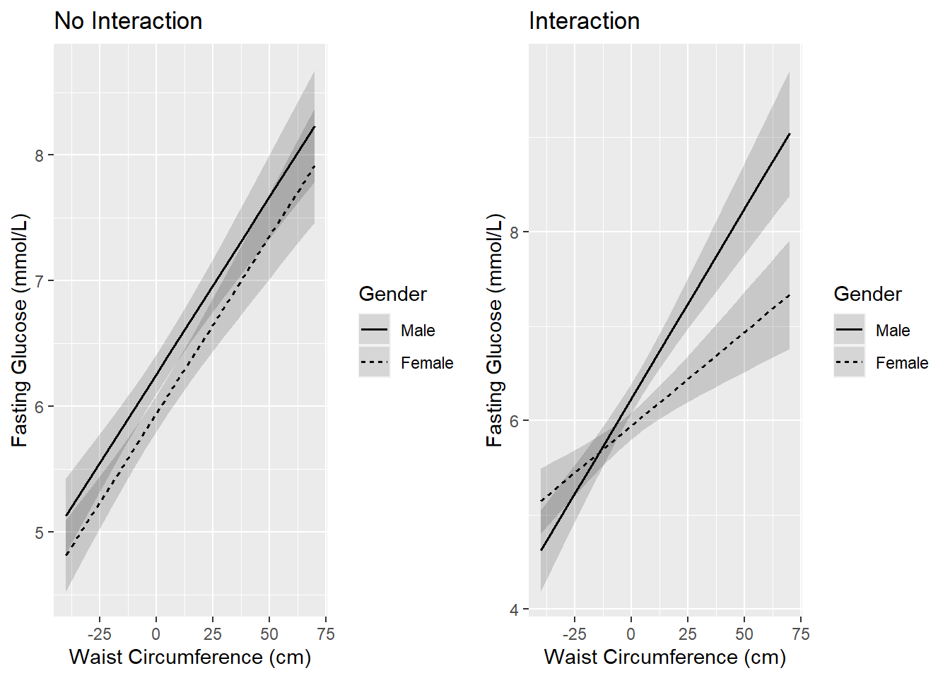
Figure 5.15: Linear regression interaction plot (continuous x categorical)
Although it is a subjective judgment, visually it appears that the interaction is meaningfully large. In the next section, we will test to see if the magnitude of the interaction is statistically significant.
5.10.6 Testing the difference between the slopes
In the right panel of Figure 5.15, is the difference between the male and female slopes statistically significant? This is equivalent to asking, “Are the lines in the plot significantly different from parallel?” Recall the regression equation for this interaction model.
\[ \textrm{FG} = \beta_0 + \beta_1 \textrm{WC} + \beta_2 I(\textrm{Gender} = \textrm{Female}) + \beta_3 [WC \times I(Gender = Female)] + \epsilon \]
The p-value for the regression coefficient for the interaction tests the null hypothesis \(H_0: \beta_3 = 0\). Under the null hypothesis, the lines are parallel. Thus, to test the difference between the slopes, examine the interaction p-value.
##                         Estimate Std. Error t value Pr(>|t|)
## (Intercept)                2.209      0.503   4.396    0.000
## BMXWAIST                   0.040      0.005   8.276    0.000
## RIAGENDRFemale             1.746      0.649   2.690    0.007
## BMXWAIST:RIAGENDRFemale   -0.020      0.006  -3.218    0.001
From the output, the p-value for the test of interaction is .001. In this case, since the interaction was between a continuous predictor and a binary predictor, the interaction is just one term, so the test can be obtained directly from the regression coefficient table. In Section 5.10.10 we will discuss what to do when the interaction involves a categorical predictor with more than two levels.
Since p < .05, we can make the following two inferences:
- There is a significant difference in the WC effect on fasting glucose between males and females (the lines are significantly different from parallel).
- There is a significant difference in the gender effect on fasting glucose between those with differing WC (the vertical distance between the lines depends on how large or small WC is).
5.10.7 Estimating and testing the significance of the slope at each level of a moderator
We just showed that the WC effect is significantly greater for males than for females. What if you want to estimate and test the significance of the WC effect for each gender individually (testing whether the line for males is significantly different from a horizontal line and, separately, testing whether the line for females is significantly different from a horizontal line)?
The null hypothesis for the test of the WC effect among males is a test of the slope for males, \(H_0: \beta_1=0\). Since this involves just one regression coefficient, you can read this right off the output in the BMXWAIST row of the COEFFICIENTS table since that row corresponds to \(\beta_1\). Thus, the WC effect for males is statistically significant (B = 0.040; 95% CI = 0.031, 0.050; p <.001).
However, the slope for females is the sum of two regression coefficients (\(\beta_1 + \beta_3\)). How do we conduct the test for females? You could re-fit the model after setting “Female” to be the reference level instead of “Male”. In this new model, the WC main effect would be the slope for females. However there is a more generally applicable method that is useful to learn and does not involve re-fitting the model.
In our current model, in which “Male” was the reference level for gender, the test of the WC effect among females is \(H_0: \beta_1 + \beta_3 = 0\). The function gmodels::estimable() (Warnes et al. 2022) can be used to estimate and test any linear combination of regression coefficients. To use this function with a model with four regression coefficients (including the intercept), specify a vector \((a, b, c, d)\) corresponding to the linear combination \(a\beta_0 + b\beta_1 + c\beta_2 + d\beta_3\) of interest. The function will then estimate this sum and test the null hypothesis that it is 0. For females, since we want to test \(\beta_1 + \beta_3\), our vector is \((0, 1, 0, 1)\).
NOTE: When using gmodels::estimable() to estimate the effect of \(X\) at levels of \(Z\), always include a 1 in the slot for the main effect of \(X\), do not include a 1 for the main effect of \(Z\), and include the value of \(Z\) in the slot for the \(X \times Z\) interaction. In this example, \(X\) is WC and \(Z\) is \(I(\textrm{Gender} = \textrm{Female})\), so we include a 1 in the WC main effect slot (slot 2) and a 1 or 0 in the interaction slot (slot 4) depending on whether gender is female or male.
To make sure you are putting the numbers in the correct slots, look at the number, order, and spelling of the coefficients in the lm object. In the code below, the vector specifying the linear combination is a named vector. The names are not required but are a good idea to ensure the correct numbers are entered in the correct slots.
## [1] 4# Select the 1st column
# Include drop=F to keep it as a matrix (which displays vertically)
summary(fit.ex5.2.int)$coef[, 1, drop=F]## Estimate
## (Intercept) 2.20932
## BMXWAIST 0.04024
## RIAGENDRFemale 1.74592
## BMXWAIST:RIAGENDRFemale -0.02036# Test slope for females
gmodels::estimable(fit.ex5.2.int,
c("(Intercept)" = 0,
"BMXWAIST" = 1,
"RIAGENDRFemale" = 0,
"BMXWAIST:RIAGENDRFemale" = 1),
conf.int = 0.95)## Estimate Std. Error t value DF Pr(>|t|) Lower.CI Upper.CI
## (0 1 0 1) 0.01988 0.004051 4.907 853 0.000001106 0.01193 0.02783Any terms omitted will be assumed to be multiplied by zero. Thus, the following abbreviated code produces the same result.
gmodels::estimable(fit.ex5.2.int,
                   c("BMXWAIST"                = 1,
                     "BMXWAIST:RIAGENDRFemale" = 1),
                   conf.int = 0.95)
You can also get the same answer without naming the terms, but then you must include all the slots. However, use this method with caution as without names it is easy to enter values in the wrong slots.
Although we already tested the slope for males above, we could use gmodels::estimable() instead. For males, the vector would be \((0, 1, 0, 0)\) (to test \(H_0: \beta_1=0\)).
# Test slope for males
# Optionally, round the output
round(
  gmodels::estimable(fit.ex5.2.int,
                   c("(Intercept)"             = 0,
                     "BMXWAIST"                = 1,
                     "RIAGENDRFemale"          = 0,
                     "BMXWAIST:RIAGENDRFemale" = 0),
                   conf.int = 0.95)
, 4)
## Estimate Std. Error t value DF Pr(>|t|) Lower.CI Upper.CI
## (0 1 0 0) 0.0402 0.0049 8.276 853 0 0.0307 0.0498Conclusion: The WC effects for males (Est = 0.040; 95% CI = 0.031, 0.050; p <.001) and females (Est = 0.020; 95% CI = 0.012, 0.028; p <.001) are statistically significant.
5.10.8 A two-way interaction has two interpretations
Above, we saw how the WC effect differed by gender. We can also break down the regression equation by WC to see how the gender effect differs by WC. Let’s see what the equations look like at WC = 80, 100, and 120 cm.
To get the regression equation at WC = 80, plug this value into Equation (5.2) to get the following.
\[\begin{array}{rcl} E(\textrm{FG} | \textrm{WC} = 80, \textrm{Gender}) & = & 2.209 \\ & + & 0.040 \times 80 \\ & - & 1.746 \times I(\textrm{Gender} = \textrm{Female}) \\ & - & 0.020 \times 80 \times I(\textrm{Gender} = \textrm{Female}) \end{array}\]
which reduces to
\[ E(\textrm{FG} │ \textrm{WC}=80, \textrm{Gender}) = 5.429 + 0.117 \times I(\textrm{Gender}=\textrm{Female}) \]
The math was carried out before rounding so you may get a different answer if you start with the values rounded to three digits. Similarly, for the other WC values, we get the following.
\[\begin{array}{rcl} E(\textrm{FG} │ \textrm{WC}=100, \textrm{Gender}) & = & 6.233 - 0.290 \times I(\textrm{Gender}=\textrm{Female}) \\ E(\textrm{FG} │ \textrm{WC}=120, \textrm{Gender}) & = & 7.038 - 0.698 \times I(\textrm{Gender}=\textrm{Female}) \end{array}\]
As WC increases from 80 to 120 cm (a total of 40 cm), the gender effect changes by 40 \(\times\) the interaction effect, or \(40 \times -0.0204= -0.8145\), going from 0.117 to -0.698. Visualize this by looking at how far apart the Male and Female regression lines are at different WC values, as shown in Figure 5.16.
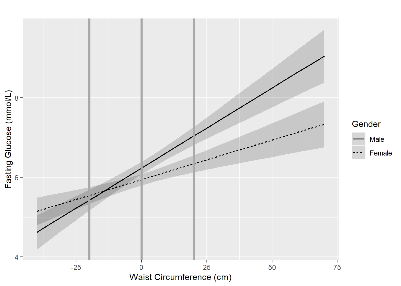
Figure 5.16: Gender effect depends on waist circumference
Another interaction plot that shows the effect of RIAGENDR at each level of BMXWAIST can be created using plot_model() with the terms reversed as terms = c("RIAGENDR", "BMXWAIST") (Figure 5.17). By default, if the second term is continuous, the effect of the first will be shown at the following values of the second: mean – 1 standard deviation, mean, mean + 1 standard deviation. To specify different values (e.g., 80, 100, 120), use the syntax below.
plot_model(fit.ex5.2.int,
           type = "eff",
           terms = c("RIAGENDR", "BMXWAIST [80, 100, 120]"),
           axis.title = c("Gender",
                          "Fasting Glucose (mmol/L)"),
           legend.title = "Waist Circumference(cm)",
           title = "")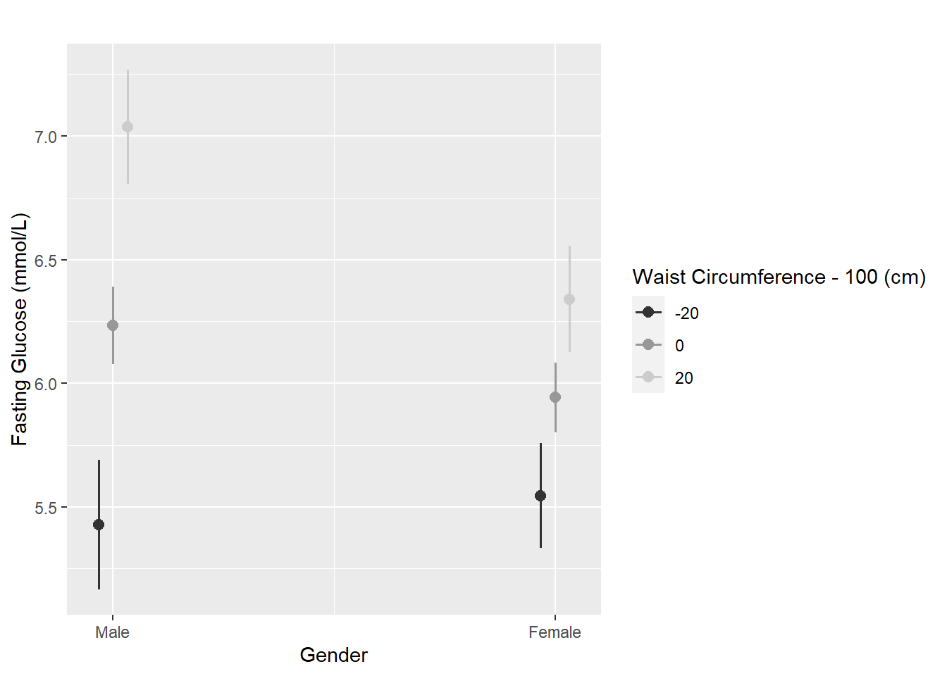
Figure 5.17: Another way of seeing that the gender effect depends on waist circumference
Conclusion: The magnitude of the association between WC and fasting glucose differs significantly between males and females (p = .001) (this is the p-value for the interaction). The association between WC and fasting glucose is significant for both males (Slope = 0.040; 95% CI = 0.031, 0.050; p <.001) and females (Slope = 0.020; 95% CI = 0.012, 0.028; p <.001), but is significantly lower for females (B-interaction (difference in slopes) = -0.020; 95% CI = -0.033, -0.008; p = .001).
If you feel confused by interactions, you are not alone! Assuming your confusion is not due to the author’s lack of clarity, take comfort in the fact that interactions are inherently tricky, but you will learn and get used to them with experience. They are easy to misunderstand and misinterpret, so if you feel confused that is a good thing in one respect – it means you know enough to be careful and ask for help until you are comfortable dealing with interactions on your own.
5.10.9 Types of two-way interactions
In regression, you can have the following different kinds of two-way interactions:
- Interaction between a continuous predictor and a categorical predictor
- Interaction between two categorical predictors
- Interaction between two continuous predictors
5.10.9.1 Continuous \(\times\) categorical
This is the type of interaction discussed in Example 5.2 in Sections 5.10.1 to 5.10.8 (WC \(\times\) gender).
5.10.9.2 Categorical \(\times\) categorical
An interaction between two categorical predictors can be more complicated. For example, if you have a categorical predictor with 2 levels interacted with a categorical predictor with 3 levels, you do not have two regression lines but rather 2 \(\times\) 3 = 6 means. In addition, it is possible that even if neither predictor was sparse enough to warrant collapsing levels, one or the other might be sparse within levels of the other.
Example 5.3 Regress fasting glucose on gender and income, along with their interaction, interpret the regression coefficients, and visualize the interaction.
First, check to see if any combination of these predictors is sparse.
##
##          <$25,000 $25,000 to <$55,000 $55,000+
##   Male         67                 106      215
##   Female       90                 115      264
All combinations have relatively large sample sizes. If some combination had a very small sample size, then one or more of the interaction terms would be estimated very imprecisely. In that case, it might be a good idea to collapse one or more of the predictors involved in the interaction (see Section 5.4.5).
The syntax for fitting this model is the same as for the continuous \(\times\) categorical model.
fit.ex5.3.int <- lm(LBDGLUSI ~ RIAGENDR + income +
                      RIAGENDR:income,
                    data = nhanesf.complete)
round(summary(fit.ex5.3.int)$coef, 3)
## Estimate Std. Error t value Pr(>|t|)
## (Intercept) 6.233 0.199 31.266 0.000
## RIAGENDRFemale 0.216 0.263 0.820 0.413
## income$25,000 to <$55,000 0.101 0.255 0.396 0.693
## income$55,000+ 0.102 0.228 0.447 0.655
## RIAGENDRFemale:income$25,000 to <$55,000 -0.712 0.343 -2.077 0.038
## RIAGENDRFemale:income$55,000+ -0.742 0.303 -2.448 0.015Including the intercept, there are six coefficients above. These can be combined to estimate mean fasting glucose at the six possible combinations of gender \(\times\) income. Let’s compute the mean at each level. We could use gmodels::estimable() but for estimating the mean outcome at levels of categorical predictors (as opposed to the slopes of continuous predictors, which are not estimated means) using predict() is much easier.
# Get levels of each categorical predictors
LEVELS1 <- levels(nhanesf.complete$income)
LEVELS2 <- levels(nhanesf.complete$RIAGENDR)

# Create a data.frame to store the predictions
preddat <- data.frame(
  income   = rep(LEVELS1, length(LEVELS2)),
  RIAGENDR = rep(LEVELS2, each=length(LEVELS1))
)

# Add the predictions
preddat$pred <- predict(fit.ex5.3.int, preddat)

# View the predicted means
preddat
## income RIAGENDR pred
## 1 <$25,000 Male 6.233
## 2 $25,000 to <$55,000 Male 6.334
## 3 $55,000+ Male 6.335
## 4 <$25,000 Female 6.449
## 5 $25,000 to <$55,000 Female 5.837
## 6 $55,000+ Female 5.809We can also visualize these means using plot_model(), as shown in Figure 5.18.
plot_model(fit.ex5.3.int,
           type = "eff",
           terms = c("income", "RIAGENDR"),
           axis.title = c("Income",
                          "Fasting Glucose (mmol/L)"),
           title = "")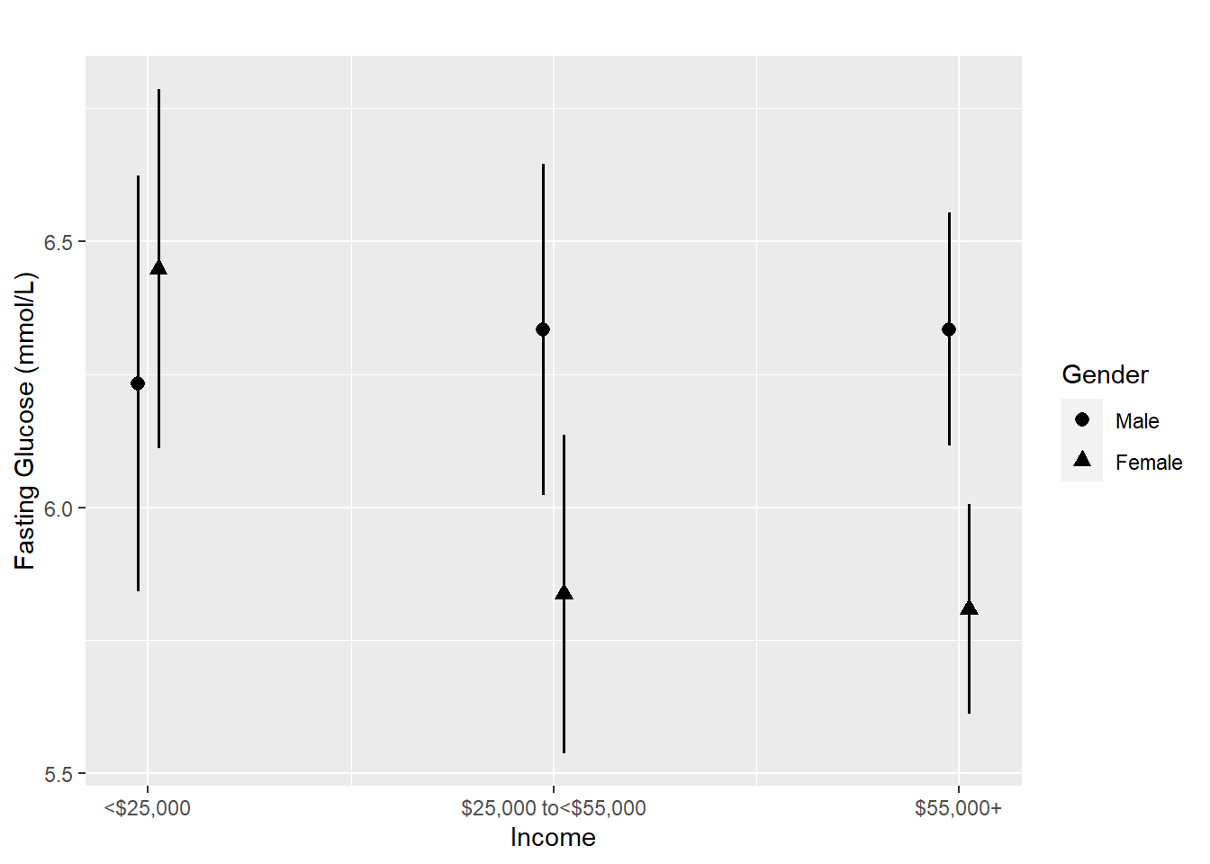
Figure 5.18: Interaction of two categorical predictors: Fasting Glucose vs. Income by Gender
Is the interaction statistically significant? When you have an interaction between categorical predictors with \(L_1\) and \(L_2\) levels, there will be \((L_1-1) \times (L_2-1)\) interaction terms. If this product is >1, which it will be if either categorical predictor has more than two levels, then you cannot get this test from the default lm() output since it is a multiple degree of freedom test (you are testing more than one coefficient simultaneously). But you can get it using car::Anova().
## Anova Table (Type III tests)
##
## Response: LBDGLUSI
##                 Sum Sq  Df F value              Pr(>F)
## (Intercept)       2603   1  977.55 <0.0000000000000002 ***
## RIAGENDR             2   1    0.67               0.413
## income               1   2    0.11               0.898
## RIAGENDR:income     17   2    3.17               0.042 *
## Residuals         2266 851
## ---
## Signif. codes:  0 '***' 0.001 '**' 0.01 '*' 0.05 '.' 0.1 ' ' 1
We conclude that there is a statistically significant interaction between gender and income (p = .042). From Figure 5.18, we see that females have a greater mean fasting glucose among those with income <$25,000 but a lower mean fasting glucose among those with income \(\ge\)$25,000.
What if you want to estimate the difference between specific levels of one predictor at a certain level of the other?
For example, estimate the difference in mean fasting glucose between males and females among those with different incomes.
- The main effect regression coefficient for
RIAGENDRFemaleis the difference in mean fasting glucose between females and males at the reference level of income, which is <$25,000. - The difference in mean outcome between females and males among those making $25,000 to <$55,000 is the sum of the
RIAGENDRFemalemain effect and theRIAGENDRFemale:income$25,000 to <$55,000interaction term. - The difference in mean outcome between females and males among those making $55,000+ is the sum of the
RIAGENDRFemalemain effect and theRIAGENDRFemale:income$55,000+interaction term.
Since these are sums of coefficients, use gmodels::estimable() to estimate these effects. First, look at the coefficient vector to confirm the number, order, and spelling of the terms in the model.
## [1] 6## Estimate
## (Intercept) 6.2328
## RIAGENDRFemale 0.2158
## income$25,000 to <$55,000 0.1007
## income$55,000+ 0.1021
## RIAGENDRFemale:income$25,000 to <$55,000 -0.7122
## RIAGENDRFemale:income$55,000+ -0.7418There are six slots. The gender main effect is RIAGENDRFemale and the interaction terms are RIAGENDRFemale:income$25,000 to <$55,000 and RIAGENDRFemale:income$55,000+. Since we are estimating gender effects at levels of income, always assign a 1 to the gender main effect slot, and assign a 0 or 1 to each interaction term, depending on the level of income.
rbind(
  # Females vs. Males, Income <$25,000
  # (income reference level, so no 1 in any interaction slot)
  gmodels::estimable(fit.ex5.3.int,
                     c("RIAGENDRFemale" = 1),
                     conf.int = 0.95),
  # Females vs. Males, Income $25,000 to <$55,000
  gmodels::estimable(fit.ex5.3.int,
                     c("RIAGENDRFemale" = 1,
                       "RIAGENDRFemale:income$25,000 to <$55,000" = 1),
                     conf.int = 0.95),
  # Females vs. Males, Income $55,000+
  gmodels::estimable(fit.ex5.3.int,
                     c("RIAGENDRFemale" = 1,
                       "RIAGENDRFemale:income$55,000+" = 1),
                     conf.int = 0.95)
)
## Estimate Std. Error t value DF Pr(>|t|) Lower.CI Upper.CI
## (0 1 0 0 0 0) 0.2158 0.2633 0.8197 851 0.4126023 -0.3010 0.73262
## (0 1 0 0 1 0) -0.4964 0.2197 -2.2592 851 0.0241231 -0.9276 -0.06513
## (0 1 0 0 0 1) -0.5260 0.1499 -3.5087 851 0.0004739 -0.8202 -0.23174Equivalently, you could use the following code. It is a matter of preference which form you use. The former is less error-prone in that the slots are named and you do not have to keep track of the position of the slots. Also, the former is more intuitive if you understand what is needed as “main effect + an interaction term”. However, the latter is nice in that it is easy to see the similarities and differences between the three vectors since they are lined up. They all have a 1 in the main effect slot, the first has no 1 in any interaction slot, and the remaining have a 1 in consecutive interaction slots.
rbind(
  gmodels::estimable(fit.ex5.3.int, c(0, 1, 0, 0, 0, 0), conf.int = 0.95),
  gmodels::estimable(fit.ex5.3.int, c(0, 1, 0, 0, 1, 0), conf.int = 0.95),
  gmodels::estimable(fit.ex5.3.int, c(0, 1, 0, 0, 0, 1), conf.int = 0.95)
)
Conclusion:
- Among those making <$25,000 per year, fasting glucose is greater in females than males, although this difference is not statistically significant (Est = 0.22; 95% CI = -0.30, 0.73; p = .413).
- Among those making $25,000 to <$55,000 per year, fasting glucose is significantly lower in females than males (Est = -0.50; 95% CI = -0.93, -0.07; p = .024).
- Among those making $55,000 or more per year, fasting glucose is significantly lower in females than males (Est = -0.53; 95% CI = -0.82, -0.23; p <.001).
5.10.9.3 Continuous \(\times\) continuous
An interaction between two continuous predictors is simpler in one way but more complicated in another. It will always involve just one regression coefficient, but the relationship cannot be completely visualized as a set of regression lines since each predictor is continuous, with more than just a few possible values. However, to partially illustrate the interaction, you can plot a regression line for one predictor at a set of specific values of the other (like we did for the continuous \(\times\) categorical interaction).
Example 5.4: Regress fasting glucose on the continuous predictors waist circumference and age, along with their interaction, and interpret the regression coefficients. After fitting the model, visualize the association between waist circumference and fasting glucose for those ages 30, 40, and 50 years.
The regression equation is
\[\textrm{FG} = \beta_0 + \beta_1 \textrm{Age} + \beta_2 \textrm{WC} + \beta_3 (\textrm{Age} \times \textrm{WC}) + \epsilon\]
and the interpretation of each parameter is as follows.
- \(\beta_0\) is the mean fasting glucose among those age 0 years with WC = 0 cm.
- \(\beta_1\) is the age effect among those with WC = 0 cm. Because there is an Age \(\times\) WC interaction, the “age effect” varies with WC.
- \(\beta_2\) is the WC effect among those age 0 years. Because there is an Age \(\times\) WC interaction, the “WC effect” varies with age.
- \(\beta_3\) is the interaction effect. It represents the difference in the age effect for every cm of WC away from 0 cm, and the difference in the WC effect for every year of age away from 0 years.
Fitting the model is no different than with other forms of interactions.
# Fit model
fit.ex5.4.int <- lm(LBDGLUSI ~ RIDAGEYR + BMXWAIST +
                      RIDAGEYR:BMXWAIST,
                    data = nhanesf.complete)

# View output
round(summary(fit.ex5.4.int)$coef, 4)
## Estimate Std. Error t value Pr(>|t|)
## (Intercept) 4.8462 0.8924 5.4307 0.0000
## RIDAGEYR -0.0320 0.0191 -1.6790 0.0935
## BMXWAIST 0.0015 0.0089 0.1709 0.8644
## RIDAGEYR:BMXWAIST 0.0005 0.0002 2.9033 0.0038As mentioned, the interaction is a single term in the model so the test of significance of the interaction can be read right off the output (interaction p = .004). That is the simple aspect of a continuous \(\times\) continuous interaction. The complicated aspect is that to visualize this model we must choose a few specific values of one predictor and plot the regression lines for the other predictor at those levels. This is what we did for a continuous \(\times\) categorical interaction, but in that case there were a finite number of categorical levels; here, there are an infinite number of values you can pick from, so for this example a few interesting values were chosen (ages 30, 40, and 50 years).
Visualize the interaction using plot_model(), as shown in Figure 5.19.
plot_model(fit.ex5.4.int,
type = "eff",
terms = c("BMXWAIST", "RIDAGEYR [30, 40, 50]"),
axis.title = c("Waist Circumference (cm)",
"Fasting Glucose (mmol/L)"),
legend.title = "Age (years)",
title = "")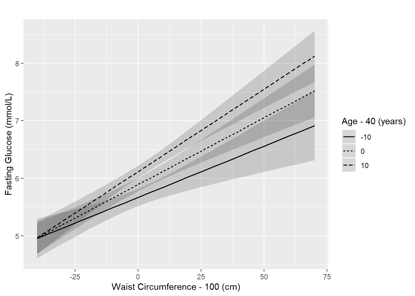
Figure 5.19: Interaction of two continuous predictors: fasting glucose vs. waist circumference, by age
Recall that the regression coefficient table is the following.
##                   Estimate Std. Error t value Pr(>|t|)
## (Intercept)         4.8462     0.8924  5.4307   0.0000
## RIDAGEYR           -0.0320     0.0191 -1.6790   0.0935
## BMXWAIST            0.0015     0.0089  0.1709   0.8644
## RIDAGEYR:BMXWAIST 0.0005 0.0002 2.9033 0.0038We can interpret the numbers in this table in light of Figure 5.19.
- The coefficient for
BMXWAISTis 0.0015. This is the slope for fasting glucose vs. WC when Age = 0 years. - The interaction term is statistically significant (p = .004). Thus, we can reject the null hypothesis that the lines are parallel, and conclude that the age effect varies with WC, and the WC effect varies with age.
- The interaction term is positive (0.0005). This means that
- the slopes for fasting glucose vs. WC at ages 30, 40, and 50 years are 0.0015 + 30 \(\times\) 0.0005, 0.0015 + 40 \(\times\) 0.0005, and 0.0015 + 50 \(\times\) 0.0005, respectively;
- the slope is larger among those who are older, as can be seen by the fact that lines become more steep at older age; and
- differences in fasting glucose between those of different ages are greater among those with greater WC (the lines are further apart for larger WC values).
What if you want to estimate the WC slopes at each of these ages?
The WC slope at a given age is the BMXWAIST main effect plus age times the RIDAGEYR:BMXWAIST interaction. Use gmodels::estimable() to estimate these effects. First, look at the coefficient vector to confirm the number, order, and spelling of the terms in the model.
## [1] 4## Estimate
## (Intercept) 4.8462057
## RIDAGEYR -0.0319988
## BMXWAIST 0.0015185
## RIDAGEYR:BMXWAIST 0.0005434There are four slots. The WC main effect is in slot 3, and the interaction term is in slot 4. While we still enter a 1 in the main effect slot (as in all our previous examples), in the interaction slot we enter the age value rather than a 1 (since age is continuous).
round(rbind(
gmodels::estimable(fit.ex5.4.int,
c("BMXWAIST" = 1,
"RIDAGEYR:BMXWAIST" = 30),
conf.int = 0.95),
gmodels::estimable(fit.ex5.4.int,
c("BMXWAIST" = 1,
"RIDAGEYR:BMXWAIST" = 40),
conf.int = 0.95),
gmodels::estimable(fit.ex5.4.int,
c("BMXWAIST" = 1,
"RIDAGEYR:BMXWAIST" = 50),
conf.int = 0.95)
), 6)## Estimate Std. Error t value DF Pr(>|t|) Lower.CI Upper.CI
## (0 0 1 30) 0.01782 0.004105 4.340 853 0.000016 0.009761 0.02588
## (0 0 1 40) 0.02325 0.003186 7.297 853 0.000000 0.016998 0.02951
## (0 0 1 50) 0.02869 0.003234 8.871 853 0.000000 0.022339 0.03503Conclusion:
- Among those age 30 years, those with 1-unit greater WC have, on average, a fasting glucose that is 0.0178 greater (Est = 0.0178; 95% CI = 0.0098, 0.0259; p <.001).
- Among those age 40 years, those with 1-unit greater WC have, on average, a fasting glucose that is 0.0233 greater (Est = 0.0233; 95% CI = 0.0170, 0.0295; p <.001).
- Among those age 50 years, those with 1-unit greater WC have, on average, a fasting glucose that is 0.0287 greater (Est = 0.0287; 95% CI = 0.0223, 0.0350; p <.001).
5.10.10 Test of interaction
This section reviews the methods for carrying out a test of significance of the interaction term. We already carried out this test for each type of interaction in the previous sections, but the method is summarized here.
For a regression with outcome \(Y\) and an interaction between \(X\) and \(Z\), a statistical test of interaction is a test of the null hypothesis that the magnitude of the effect of \(X\) on \(Y\) does not depend on \(Z\), and that the magnitude of the effect of \(Z\) on \(Y\) does not depend on \(X\). Visually, the null hypothesis corresponds to parallel lines in plots such as Figures 5.15 and 5.19. Statistically, the null hypothesis is that all the regression coefficients that define the interaction are zero.
When the interaction involves just one term in the model (one row in the regression coefficient table) you can get the p-value for the interaction test by looking at the regression table. For example, if the regression formula is \(Y = \beta_0 + \beta_1 X + \beta_2 Z + \beta_3 XZ + \epsilon\), the null hypothesis is \(H_0: \beta_3 = 0\). In our example of an interaction between two continuous predictors, we would look in the row with the term that contains a : (RIDAGEYR:BMXWAIST).
##                   Estimate Std. Error t value Pr(>|t|)
## (Intercept)         4.8462     0.8924  5.4307   0.0000
## RIDAGEYR           -0.0320     0.0191 -1.6790   0.0935
## BMXWAIST            0.0015     0.0089  0.1709   0.8644
## RIDAGEYR:BMXWAIST 0.0005 0.0002 2.9033 0.0038When at least one of the terms in the interaction is a categorical predictor with more than two levels, the interaction will consist of multiple terms. For example, if \(Z\) is categorical with levels 1 (the reference level), 2, and 3, the regression formula is
\[Y = \beta_0 + \beta_1 X + \beta_2 I(Z=2) + \beta_3 I(Z=3) + \beta_4 X \times I(Z=2) + \beta_5 X \times I(Z=3) + \epsilon\]
and the null hypothesis of no interaction is \(H_0: \beta_4 = 0 \textrm{ and } \beta_5 = 0\). In our example of an interaction between two categorical predictors, one of which had more than two levels, the rows with the : terms do not provide the interaction test, as they are tests of each of the interaction terms individually. The estimated regression coefficients were:
##                                          Estimate Std. Error t value Pr(>|t|)
## (Intercept)                                6.2328     0.1994 31.2658   0.0000
## RIAGENDRFemale                             0.2158     0.2633  0.8197   0.4126
## income$25,000 to <$55,000                  0.1007     0.2547  0.3956   0.6925
## income$55,000+                             0.1021     0.2283  0.4472   0.6549
## RIAGENDRFemale:income$25,000 to <$55,000  -0.7122     0.3429 -2.0768   0.0381
## RIAGENDRFemale:income$55,000+             -0.7418     0.3030 -2.4483   0.0146
Recall that to test the main effect for a categorical predictor with more than two levels, we used car::Anova() to carry out the multiple df test. We can do the same for a multiple df interaction:
## Anova Table (Type III tests)
##
## Response: LBDGLUSI
##                 Sum Sq  Df F value              Pr(>F)
## (Intercept)       2603   1  977.55 <0.0000000000000002 ***
## RIAGENDR             2   1    0.67               0.413
## income               1   2    0.11               0.898
## RIAGENDR:income     17   2    3.17               0.042 *
## Residuals         2266 851
## ---
## Signif. codes:  0 '***' 0.001 '**' 0.01 '*' 0.05 '.' 0.1 ' ' 1
We conclude for this example that there is a significant gender \(\times\) income interaction (F[2, 851] = 3.17, p = .042). The same method (car::Anova()) would be used for a continuous \(\times\) categorical interaction if the categorical predictor has more than two levels.
By way of reminder, the tests of each of the two main effects are not tests of the overall effect of each of the corresponding predictors. They are, rather, tests of significance of each predictor at the reference level of the other predictor in the interaction. The following subsection will discuss how to obtain an appropriate overall test for each predictor involved in an interaction.
5.10.11 Overall test of a predictor involved in an interaction
In Section 5.10.10, we assessed the significance of an interaction with a test of the null hypothesis that one predictor effect does not vary with another predictor. A test of interaction answers a question such as, “Does the effect of waist circumference on fasting glucose depend on gender?”
But what if we want to answer the question, “Is waist circumference significantly associated with fasting glucose?” in a model which contains WC interacted with another predictor? This is a comparison of two models – one that includes WC and one that does not. When there is no interaction, this would simply be a test of the WC regression coefficient. When there is an interaction, however, this is a simultaneous test of the WC main effect and the WC interaction with the other predictor.
For example, if the model is
\[\textrm{FG} = \beta_0 + \beta_1 \textrm{WC} + \beta_2 I(\textrm{Gender} = \textrm{Female}) + \beta_3 [\textrm{WC} \times I(\textrm{Gender} = \textrm{Female})] + \epsilon\]
the null hypothesis we would like to test is \(H_0: \beta_1 = 0\) and \(\beta_3 = 0\). We cannot use car::Anova() for this test because these coefficients are from different terms in the model. Instead, to carry out this test, use anova() (lowercase a), which compares two nested models: a full model compared to a reduced model with some terms from the full model removed. In this example, we want to compare the full model (with both main effects and the interaction) to the model that does not have WC at all (excludes both the WC main effect and the interaction, but retains the gender main effect). Even though there are no cases with missing values in nhanesf.complete, the code subset = complete.cases(BMXWAIST) is added here in case, in the future, you imitate this code for an example in which you have not removed cases with missing values. This option ensures that fit0 is fit to the same sample as was used when fitting the full model (those with no missing values for any of the analysis variables).
# Fit the reduced model
fit0 <- lm(LBDGLUSI ~  RIAGENDR, data = nhanesf.complete,
           subset = complete.cases(BMXWAIST))
# Compare reduced and full models
anova(fit0, fit.ex5.2.int)
## Analysis of Variance Table
##
## Model 1: LBDGLUSI ~ RIAGENDR
## Model 2: LBDGLUSI ~ BMXWAIST + RIAGENDR + BMXWAIST:RIAGENDR
## Res.Df RSS Df Sum of Sq F Pr(>F)
## 1 855 2295
## 2 853 2071 2 225 46.3 <0.0000000000000002 ***
## ---
## Signif. codes: 0 '***' 0.001 '**' 0.01 '*' 0.05 '.' 0.1 ' ' 1Thus, we conclude that the model with both WC and a WC \(\times\) gender interaction is significantly better than the model with just gender (F[2,853] = 46.3, p <.001), or that WC is significantly associated with fasting glucose.
5.10.12 When to include an interaction
If a research question is of the form “Does the association between the outcome \(Y\) and predictor \(X\) depend on (some other variable) \(Z\)?”, then the regression model used to answer the question must include an interaction between \(X\) and \(Z\). In that case, there is an a priori interaction of interest. In general, when carrying out a confirmatory analysis (see Section 5.24), use subject-matter knowledge to a priori decide which interactions to include, and then leave them in the model regardless of their statistical significance. Testing candidate interactions and only including those that are statistically significant can result in biased conclusions about statistical significance unless one uses advanced techniques to obtain valid inferences that account for the method of data exploration (Faraway 1992; Harrell 2015).
What if, rather than having specific interactions you want to test, you are interested in exploring many possible interactions, and finding a model that includes only interactions that seem meaningful? In an exploratory analysis (see Section 5.24), it is acceptable to try different interactions and include or not include them based on statistical significance and/or the magnitude of the interaction effects. It is important, if using this approach, to explicitly state you are carrying out an exploratory analysis, state what criteria you used to determine which interactions to include in your final model, and note as a limitation that the p-values for all terms in the model (both main effects and interactions) may be biased due to the fact that the final model was not prespecified and decisions regarding what terms to include were based on statistical significance and/or effect size.