8.3 Weighted descriptive statistics
There are a number of survey functions for computing weighted descriptive statistics, as well as a gtsummary (Sjoberg et al. 2021, 2025) function to conveniently create a “Table 1”. We will compute these statistics overall and by exposure or outcome.
8.3.1 Overall
Example 8.1 (continued): Compute weighted descriptive statistics that estimate values for the population represented by NHANES 2017-2018 participants with non-missing values on all our analysis variables. Since the outcome variable is fasting glucose, use the design corresponding to the fasting subsample with complete data and positive weights (design.FST.nomiss).
Examples are shown first for two variables, one continuous and one categorical. Later, we will use gtsummary to create a Table 1 of weighted descriptive statistics for all the variables.
For continuous variables, use svymean(), svyvar(), and svyquantile() to compute the weighted mean, standard deviation, median, and interquartile range, and svyhist() and svyboxplot() to plot weighted histograms and boxplots (Figures 8.1 and 8.2, respectively). When using confint() to get a 95% confidence interval, add df = degf(design) to use the design DF.
NOTE: If not using a complete case analysis and a variable has missing values, add na.rm = T to each svymean or svyvar call to avoid returning a missing value. When using confint(svymean()), the na.rm=T must go in the svymean() call, not the confint() call (e.g., confint(svymean(~X, design, na.rm=T), df = degf(design))).
# Weighted mean, standard deviation, and 95% CI
cbind(
 "wMEAN" = svymean(    ~LBDGLUSI, design.FST.nomiss),
 "wSD"   = sqrt(svyvar(~LBDGLUSI, design.FST.nomiss)[1]),
       confint(svymean(~LBDGLUSI, design.FST.nomiss), df=degf(design.FST.nomiss))
)
## wMEAN wSD 2.5 % 97.5 %
## LBDGLUSI 6.106 1.763 5.976 6.236# Weighted median, 95% CI, and standard error
# df = degf(design) is already the default for svyquantile
svyquantile(~LBDGLUSI, design.FST.nomiss, 0.50)[[1]]## quantile ci.2.5 ci.97.5 se
## 0.5 5.72 5.66 5.83 0.03988# Weighted interquartile range
c("wIQR" =
svyquantile(~LBDGLUSI, design.FST.nomiss, 0.75)[[1]][1, "quantile"] -
svyquantile(~LBDGLUSI, design.FST.nomiss, 0.25)[[1]][1, "quantile"])## wIQR
## 0.83par(mfrow=c(1,2))
# Unweighted probability histogram
hist(nhanes.mod$LBDGLUSI[nhanes.mod$nomiss], probability = T,
xlab = "Fasting Glucose (mmol/L)", main = "Unweighted",
ylim = c(0,0.35))
# Weighted probability histogram
svyhist( ~LBDGLUSI, design.FST.nomiss,
xlab = "Fasting Glucose (mmol/L)", main = "Weighted",
ylim = c(0,0.35))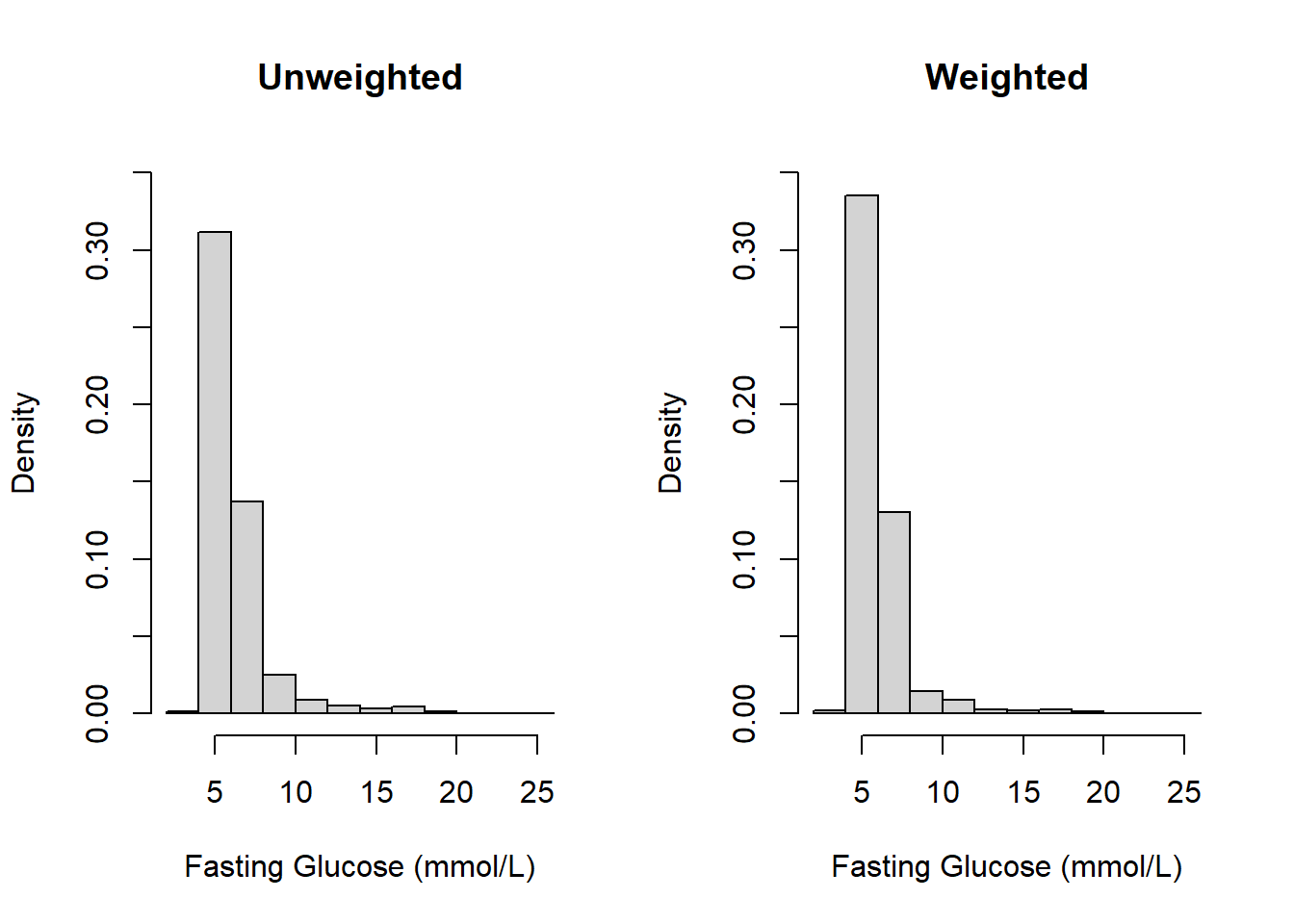
Figure 8.1: Unweighted vs. weighted histograms
par(mfrow=c(1,2))
# Unweighted boxplot
boxplot(nhanes.mod$LBDGLUSI[nhanes.mod$nomiss],
     ylab = "Fasting Glucose (mmol/L)",
     main = "Unweighted")
# Weighted boxplot
svyboxplot(~LBDGLUSI ~ 1, design.FST.nomiss, all.outliers = T,
     ylab = "Fasting Glucose (mmol/L)",
     main = "Weighted")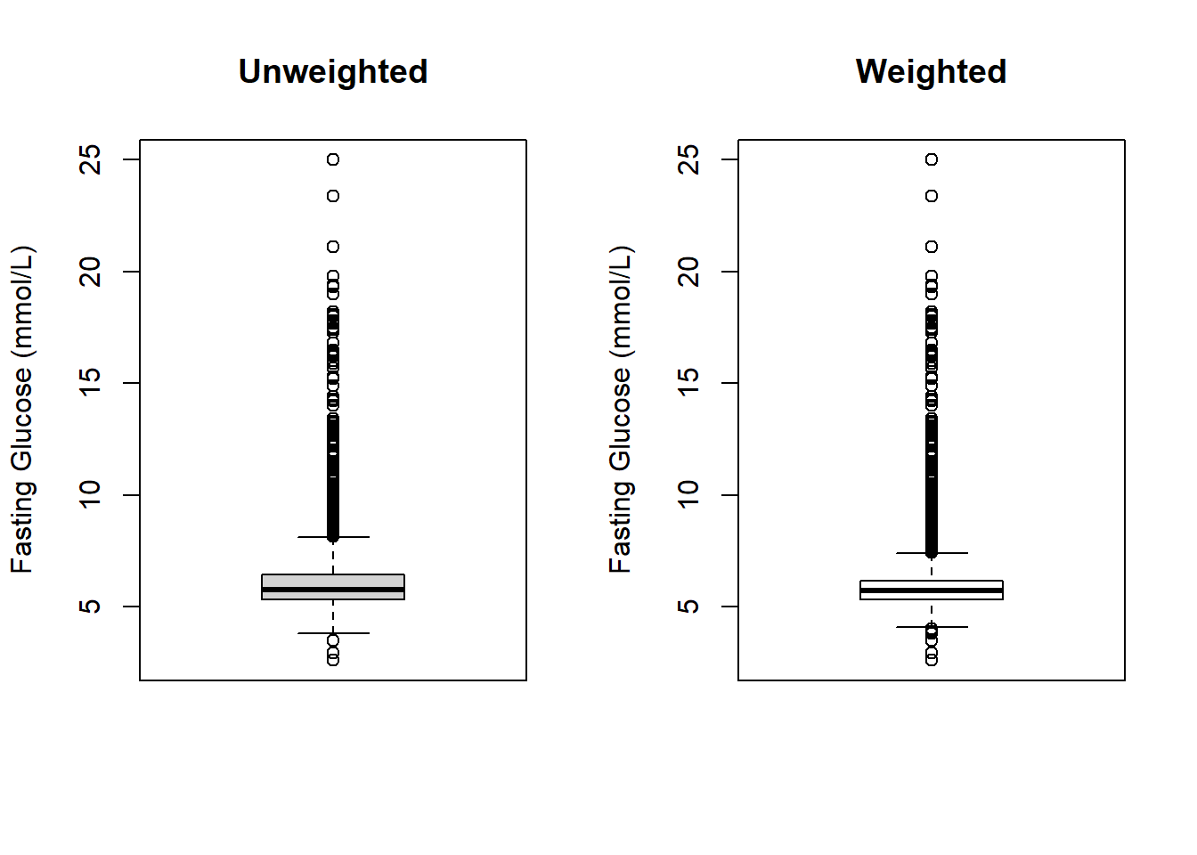
Figure 8.2: Unweighted vs. weighted boxplots
For categorical variables, use svytotal() or svytable() to estimate population totals. In a sample we compute sample frequencies, but the corresponding population quantity is a population total. Use svymean(), svytable() or svyciprop() to estimate population proportions. Use barplot() on the output of svytable() to plot a weighted barchart (Figure 8.3).
NOTE: If not using a complete case analysis and a variable has missing values, add na.rm = T to each svytotal() or svymean() call to avoid returning a missing value.
##                                total       SE
## race_ethHispanic            32712402  4552659
## race_ethNon-Hispanic White 137704704 10603571
## race_ethNon-Hispanic Black  23063852  3388626
## race_ethNon-Hispanic Other 21072543 2998573## race_eth
## Hispanic Non-Hispanic White Non-Hispanic Black Non-Hispanic Other
## 32712402 137704704 23063852 21072543## mean SE
## race_ethHispanic 0.1525 0.02
## race_ethNon-Hispanic White 0.6418 0.03
## race_ethNon-Hispanic Black 0.1075 0.02
## race_ethNon-Hispanic Other 0.0982 0.01# Weighted proportion using svytable by normalizing the total to 1
svytable(~race_eth, design.FST.nomiss, Ntotal=1)## race_eth
## Hispanic Non-Hispanic White Non-Hispanic Black Non-Hispanic Other
## 0.15247 0.64182 0.10750 0.09822# Weighted proportion with 95% CI
# df = degf(design) is already the default for svyciprop
svyciprop(~I(race_eth=="Hispanic"), design.FST.nomiss)## 2.5% 97.5%
## I(race_eth == "Hispanic") 0.152 0.113 0.203# (results for other 3 levels not shown)
svyciprop(~I(race_eth=="Non-Hispanic White"), design.FST.nomiss)
svyciprop(~I(race_eth=="Non-Hispanic Black"), design.FST.nomiss)
svyciprop(~I(race_eth=="Non-Hispanic Other"), design.FST.nomiss)par(mfrow=c(2,1))
# Unweighted barplot
barplot(prop.table(table(nhanes.mod$race_eth[nhanes.mod$nomiss])),
ylab = "Proportion", xlab = "Race/Ethnicity",
main = "Unweighted", cex.names = 0.65)
# Weighted barplot
mybar <- svytable(~race_eth, design.FST.nomiss, Ntotal=1)
barplot(mybar,
ylab = "Proportion", xlab = "Race/Ethnicity",
main = "Weighted", cex.names = 0.65)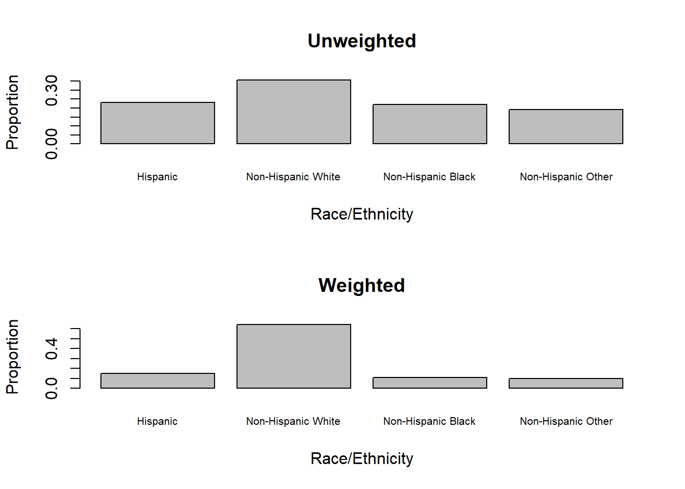
Figure 8.3: Unweighted vs. weighted barcharts
NHANES over-sampled minority groups in order to have sufficient sample sizes for subgroup analyses. Thus, there are large differences between the unweighted and weighted sample distributions of race/ethnicity, as shown in Figure 8.3. Unweighted proportions only reflect the composition of the sample, whereas weighted proportions estimate the population distribution.
Finally, use tbl_svysummary() from the gtsummary library to produce a Table 1 of weighted descriptive statistics. Instead of starting with a dataset as we did in unweighted analyses, start with the design object (design.FST.nomiss). For categorical variables, \(N\) and \(n\) values in the table are estimated population totals – when we did unweighted analyses, these were sample sizes.
The results are shown in Table 8.1.
library(gtsummary)
TABLE <- design.FST.nomiss %>%
  tbl_svysummary(
    # Use include to select variables
    include = c(LBDGLUSI, BMXWAIST, RIDAGEYR,
                smoker, RIAGENDR, race_eth, income),
    statistic = list(all_continuous()  ~ "{mean} ({sd})",
                     all_categorical() ~ "{n}    ({p}%)"),
    digits = list(LBDGLUSI ~ c(2, 2),
                  BMXWAIST ~ c(1, 1),
                  RIDAGEYR ~ c(1, 1),
                  all_categorical() ~ c(0, 1)),
    label  = list(LBDGLUSI ~ "Fasting Glucose (mmol/L)",
                  BMXWAIST ~ "Waist Circumference (cm)",
                  RIDAGEYR ~ "Age (years)",
                  smoker   ~ "Smoking Status",
                  RIAGENDR ~ "Gender",
                  race_eth ~ "Race/Ethnicity",
                  income   ~ "Annual Income")
  ) %>%
  modify_header(label = "**Variable**") %>%
  modify_caption("Weighted descriptive statistics") %>%
bold_labels()| Variable | N = 214,553,5011 |
|---|---|
| Fasting Glucose (mmol/L) | 6.11 (1.76) |
| Waist Circumference (cm) | 100.2 (17.1) |
| Age (years) | 47.0 (17.5) |
| Smoking Status | |
| Never | 123,589,210 (57.6%) |
| Past | 55,919,877 (26.1%) |
| Current | 35,044,414 (16.3%) |
| Gender | |
| Male | 104,286,253 (48.6%) |
| Female | 110,267,248 (51.4%) |
| Race/Ethnicity | |
| Hispanic | 32,712,402 (15.2%) |
| Non-Hispanic White | 137,704,704 (64.2%) |
| Non-Hispanic Black | 23,063,852 (10.7%) |
| Non-Hispanic Other | 21,072,543 (9.8%) |
| Annual Income | |
| <$25,000 | 38,141,114 (17.8%) |
| $25,000 to <$55,000 | 57,342,659 (26.7%) |
| $55,000+ | 119,069,729 (55.5%) |
| 1 Mean (SD); n (%) | |
8.3.2 By exposure or outcome
Example 8.1 (continued): Compute weighted descriptive statistics by smoking status.
For svymean(), svyvar(), svyquantile(), svytotal(), and svyciprop(), use the wrapper function svyby() to compute statistics at each level of another variable. For svytable(), however, add the by variable to the formula.
# Continuous variables, by smoking status
# Weighted mean, standard deviation, and 95% CI
WTD <- cbind(
  svyby(~LBDGLUSI, ~smoker, design.FST.nomiss, svymean)[, 1:2],
  svyby(~LBDGLUSI, ~smoker, design.FST.nomiss, svyvar)[ ,   2],
  confint(svyby(~LBDGLUSI, ~smoker, design.FST.nomiss, svymean),
          df = degf(design.FST.nomiss))
)
WTD[, 3] <- sqrt(WTD[, 3])
names(WTD)[3] <- paste(names(WTD)[2], "wSD")
names(WTD)[2] <- paste(names(WTD)[2], "wMEAN")
WTD
## smoker LBDGLUSI wMEAN LBDGLUSI wSD 2.5 % 97.5 %
## Never Never 5.965 1.543 5.796 6.135
## Past Past 6.457 2.066 6.297 6.617
## Current Current 6.041 1.894 5.798 6.285# Weighted median, standard error, and 95% CI
# df = degf(design) is already the default for svyquantile
# but not for confint
cbind(
svyby(~LBDGLUSI, ~smoker, design.FST.nomiss, svyquantile, 0.50),
confint(svyby(~LBDGLUSI, ~smoker, design.FST.nomiss, svyquantile, 0.50),
df = degf(design.FST.nomiss))
)## smoker LBDGLUSI se.LBDGLUSI 2.5 % 97.5 %
## Never Never 5.66 0.03753 5.580 5.740
## Past Past 5.83 0.03988 5.745 5.915
## Current Current 5.66 0.06568 5.520 5.800# Weighted interquartile range
Q75 <- as.data.frame(
svyby(~LBDGLUSI, ~smoker, design.FST.nomiss, svyquantile, 0.75)
)[,1:2]
Q25 <- as.data.frame(
svyby(~LBDGLUSI, ~smoker, design.FST.nomiss, svyquantile, 0.25)
)[,1:2]
names(Q75)[2] <- paste(names(Q75)[2], "wQ75")
names(Q25)[2] <- paste(names(Q25)[2], "wQ25")
WIQR <- merge(Q75, Q25)
WIQR$wIQR <- WIQR[,2] - WIQR[,3]
WIQR## smoker LBDGLUSI wQ75 LBDGLUSI wQ25 wIQR
## 1 Current 6.11 5.27 0.84
## 2 Never 6.11 5.27 0.84
## 3 Past 6.49 5.50 0.99# Categorical variables, by smoking status
# Weighted total
svytable(~race_eth + smoker, design.FST.nomiss)## smoker
## race_eth Never Past Current
## Hispanic 20524606 7861212 4326583
## Non-Hispanic White 75120526 40106079 22478099
## Non-Hispanic Black 15137153 3487312 4439386
## Non-Hispanic Other 12806924 4465273 3800346# Weighted total with SE of total
svyby(~race_eth, ~smoker, design.FST.nomiss, svytotal)
# (results not shown)Be careful when normalizing svytable() to get proportions. Using Ntotal=1 as we did previously normalizes the frequencies to the overall total. Rather, we want to normalize to the column totals to get proportions within each level of smoking status. This is accomplished using prop.table(, margin = 2). Optionally, use addmargins(, 1) to confirm that each column sums to 1.
# Weighted proportion
addmargins(
  prop.table(svytable(~race_eth + smoker, design.FST.nomiss), margin = 2)
  , 1)
## smoker
## race_eth Never Past Current
## Hispanic 0.16607 0.14058 0.12346
## Non-Hispanic White 0.60782 0.71721 0.64142
## Non-Hispanic Black 0.12248 0.06236 0.12668
## Non-Hispanic Other 0.10362 0.07985 0.10844
## Sum 1.00000 1.00000 1.00000# Weighted proportion with SE
svyby(~I(race_eth=="Hispanic"), ~smoker, design.FST.nomiss, svyciprop)## smoker I(race_eth == "Hispanic") se.as.numeric(I(race_eth == "Hispanic"))
## Never Never 0.1661 0.02650
## Past Past 0.1406 0.01976
## Current Current 0.1235 0.02512# (results for other levels not shown)
svyby(~I(race_eth=="Non-Hispanic White"), ~smoker, design.FST.nomiss, svyciprop)
svyby(~I(race_eth=="Non-Hispanic Black"), ~smoker, design.FST.nomiss, svyciprop)
svyby(~I(race_eth=="Non-Hispanic Other"), ~smoker, design.FST.nomiss, svyciprop)Finally, use tbl_svysummary() from the gtsummary library to produce a Table 1 of weighted descriptive statistics by smoking status. The results are shown in Table 8.2.
library(gtsummary)
TABLE <- design.FST.nomiss %>%
  tbl_svysummary(
    by = smoker,
    # Use include to select variables
    include = c(LBDGLUSI, BMXWAIST, RIDAGEYR,
                RIAGENDR, race_eth, income),
    statistic = list(all_continuous()  ~ "{mean} ({sd})",
                     all_categorical() ~ "{n}    ({p}%)"),
    digits = list(LBDGLUSI ~ c(2, 2),
                  BMXWAIST ~ c(1, 1),
                  RIDAGEYR ~ c(1, 1),
                  all_categorical() ~ c(0, 1)),
    label  = list(LBDGLUSI ~ "Fasting Glucose (mmol/L)",
                  BMXWAIST ~ "Waist Circumference (cm)",
                  RIDAGEYR ~ "Age (years)",
                  RIAGENDR ~ "Gender",
                  race_eth ~ "Race/Ethnicity",
                  income   ~ "Annual Income")
  ) %>%
  modify_header(label = "**Variable**",
   all_stat_cols() ~ "**{level}**<br>N = {n} ({style_percent(p, digits=1)}%)") %>%
  modify_caption("Weighted descriptive statistics, by smoking status") %>%
bold_labels()| Variable | Never N = 123589209.67615 (57.6%)1 |
Past N = 55919877.429411 (26.1%)1 |
Current N = 35044414.299371 (16.3%)1 |
|---|---|---|---|
| Fasting Glucose (mmol/L) | 5.97 (1.54) | 6.46 (2.07) | 6.04 (1.89) |
| Waist Circumference (cm) | 98.6 (17.0) | 104.0 (16.6) | 99.9 (17.4) |
| Age (years) | 45.4 (17.7) | 51.5 (18.0) | 45.4 (14.4) |
| Gender | |||
| Male | 51,169,518 (41.4%) | 34,805,126 (62.2%) | 18,311,610 (52.3%) |
| Female | 72,419,692 (58.6%) | 21,114,752 (37.8%) | 16,732,805 (47.7%) |
| Race/Ethnicity | |||
| Hispanic | 20,524,606 (16.6%) | 7,861,212 (14.1%) | 4,326,583 (12.3%) |
| Non-Hispanic White | 75,120,526 (60.8%) | 40,106,079 (71.7%) | 22,478,099 (64.1%) |
| Non-Hispanic Black | 15,137,153 (12.2%) | 3,487,312 (6.2%) | 4,439,386 (12.7%) |
| Non-Hispanic Other | 12,806,924 (10.4%) | 4,465,273 (8.0%) | 3,800,346 (10.8%) |
| Annual Income | |||
| <$25,000 | 18,081,806 (14.6%) | 9,269,756 (16.6%) | 10,789,552 (30.8%) |
| $25,000 to <$55,000 | 31,806,525 (25.7%) | 15,168,200 (27.1%) | 10,367,933 (29.6%) |
| $55,000+ | 73,700,879 (59.6%) | 31,481,921 (56.3%) | 13,886,929 (39.6%) |
| 1 Mean (SD); n (%) | |||