3.1 Examining the data
Before fitting a regression model, it is a good idea to examine each of the variables individually. One reason to do this is to look for anomalous values that may require you to look more closely at your data source. Additionally, a common element in the presentation of regression analysis results is a table containing descriptive statistics for each analysis variable.
How a variable is examined depends on whether it is continuous or categorical (as defined in Chapter 2).
- For continuous variables, create a numerical summary and plot a histogram using
summary()andhist(). - For categorical variables, create a frequency table and plot a bar chart using
table()andbarplot().
NOTE: Throughout this text, we assume that categorical variables are coded in R as factor variables (for more information, see “Factors” in R for Data Science (H. Wickham, Çetinkaya-Rundel, and Grolemund 2023) or Chapter 3 in An Introduction to R for Research (Nahhas 2024)).
Example 3.1: Using data from a random subset of 1,000 adults from the NHANES 2017-2018 examination teaching dataset (see Appendix A.1), summarize the continuous variables systolic blood pressure (sbp) and age (RIDAGEYR) and the categorical variables gender (RIAGENDR) and annual household income category (income).
First, load the NHANES examination teaching dataset using load().
load("Data/nhanes1718_adult_exam_sub_rmph.Rdata")
# For convenience, give the dataset a shorter name
nhanes <- nhanes_adult_exam_sub
Next, use summary() to look at some basic descriptive statistics for the continuous variables. None of these values seem out of the ordinary, although note that there are 42 missing values for SBP (NA's).
##    Min. 1st Qu.  Median    Mean 3rd Qu.    Max.    NA's
## 83 111 121 124 134 234 42## Min. 1st Qu. Median Mean 3rd Qu. Max.
## 20.0 32.0 47.0 47.7 61.0 80.0Use hist() to create a visualization of the entire distribution for each variable. As shown in Figure 3.1, SBP is a bit skewed to the right, which is typical for many health-related measures, and there are more younger than older individuals. There is a spike at the upper end of the age distribution because NHANES, for privacy reasons, reports ages \(\ge\) 80 years as exactly 80 years (see the NHANES documentation for RIDAGEYR, accessed May 20, 2022).
par(mfrow=c(1,2))
hist(nhanes$sbp,
     main = "",
     xlab = "Systolic Blood Pressure (mmHg)")
hist(nhanes$RIDAGEYR,
     main = "",
     xlab = "Age (years)")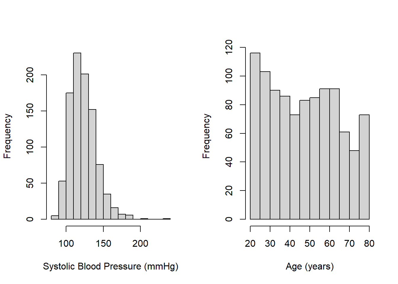
Figure 3.1: Histograms of continuous variables
Computations of common descriptive statistics are demonstrated below. The option na.rm = T is needed if there are any missing values; otherwise, the functions will return NA (indicating “missing” or “unknown”).
## [1] 123.5## [1] 17.65## [1] 121## [1] 23# 25th and 75th percentile
# (sometimes also referred to as the IQR)
quantile(nhanes$sbp,
probs = c(0.25, 0.75),
na.rm = T)## 25% 75%
## 111 134## [1] 83## [1] 234## [1] 958## [1] 42For categorical variables, use table() and prop.table() to examine the frequency and proportion of observations at each level (each possible value of a categorical variable). The useNA = "ifany" option tells R to include the number of missing values in the frequency table. In prop.table(), useNA = "ifany" is omitted here, resulting in proportions of non-missing cases.
##
##            <$25,000 $25,000 to <$55,000            $55,000+                <NA>
## 156 254 480 110##
## <$25,000 $25,000 to <$55,000 $55,000+
## 0.1753 0.2854 0.5393When a variable has no missing values, the output of table(, useNA = "ifany") simply excludes the <NA> column. To force it to appear, use table(, useNA = "always"), as demonstrated below.
##
##   Male Female   <NA>
## 482 518 0##
## Male Female
## 0.482 0.518In general, we would like to know if there are missing values. Therefore, omitting the useNA option altogether is not recommended, as that would result in exclusion of the <NA> column whether there are missing values or not. An exception is when using prop.table() to obtain the proportion of non-missing values.
The upper income group is most common and there are 110 individuals with missing income values. Missing income values are common in survey data, as some individuals are reluctant to disclose their income, even when the response options are ranges of values. Also, NHANES has gender response options “Male” and “Female” and, in this subset of the data, there are more females than males.
Options for visualizing the distribution of categorical variables include vertical and horizontal bar charts created with barplot(), as shown in Figure 3.2.
par(mfrow=c(1,2))
# barplot() expects frequencies, not the raw data, so use table inside barplot()
barplot(table(nhanes$RIAGENDR),
        ylab = "Frequency", xlab = "Gender")
barplot(table(nhanes$income), horiz=T, cex.names = 0.65,
        xlab = "Frequency", ylab = "Annual Household Income")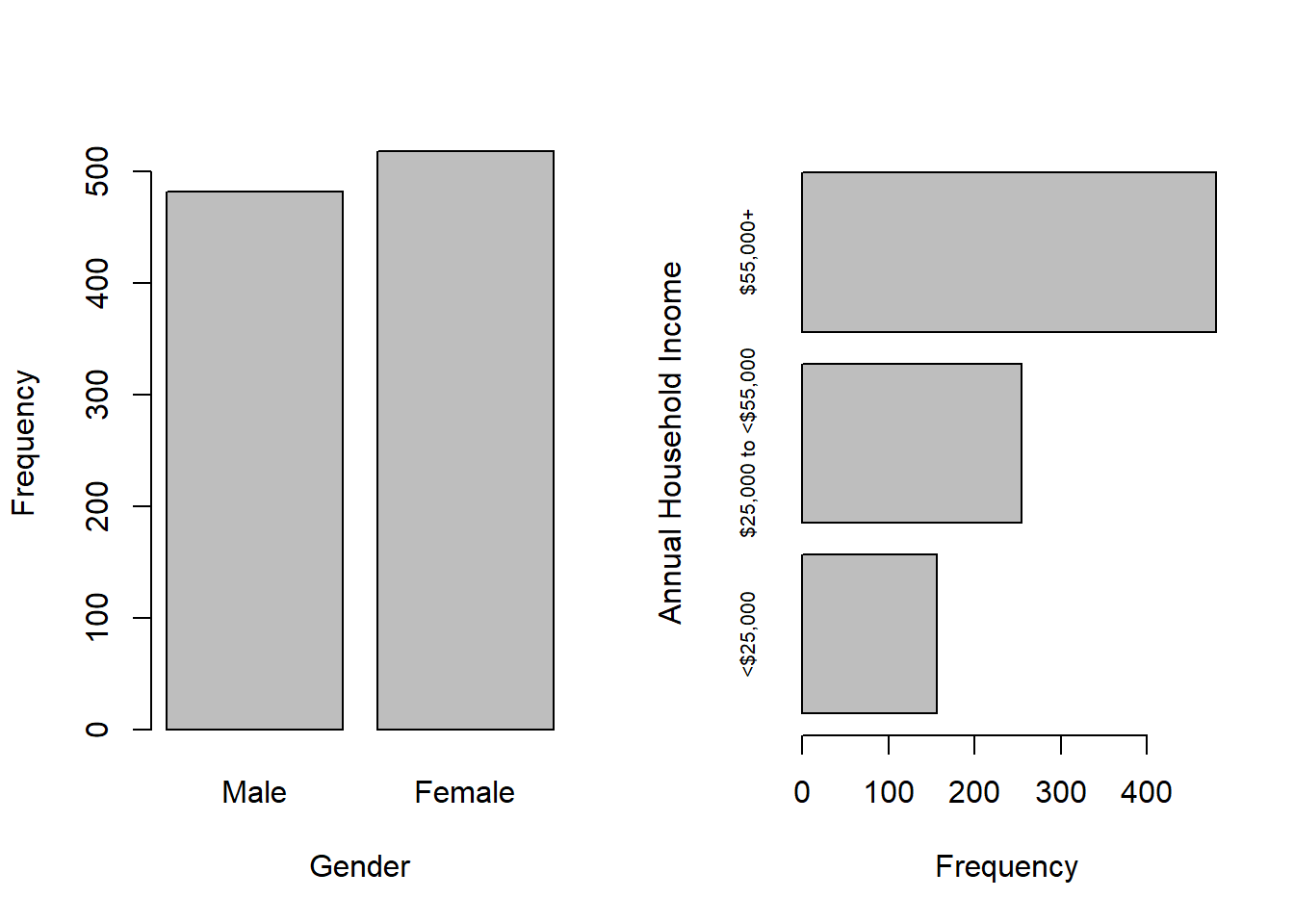
Figure 3.2: bar charts of categorical variable frequencies
Substituting prop.table(table()) for table() results in plotting proportions instead of frequencies, as shown in Figure 3.3.
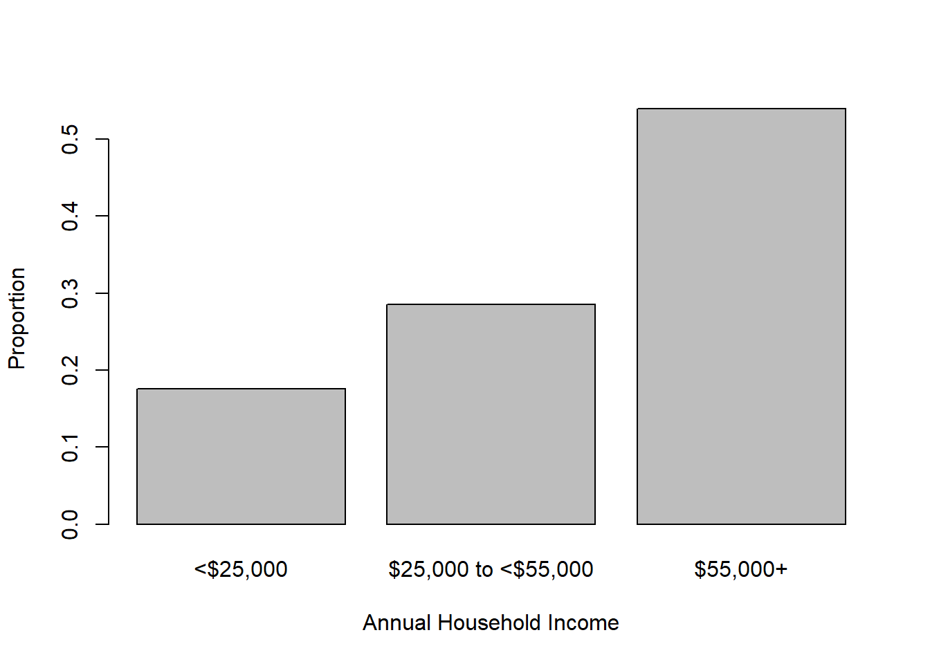
Figure 3.3: Bar chart of categorical variable proportions
3.1.1 Detailed description of all variables in a dataset
summary() can be used on multiple variables all at once, as can complete.cases().
##       sbp         RIDAGEYR      RIAGENDR                   income
##  Min.   : 83   Min.   :20.0   Male  :482   <$25,000           :156
##  1st Qu.:111   1st Qu.:32.0   Female:518   $25,000 to <$55,000:254
##  Median :121   Median :47.0                $55,000+           :480
##  Mean   :124   Mean   :47.7                NA's               :110
##  3rd Qu.:134   3rd Qu.:61.0
##  Max.   :234   Max.   :80.0
## NA's :42## [1] 1000# Number of cases with no missing data
sum(complete.cases(nhanes[, c("sbp", "RIDAGEYR", "RIAGENDR", "income")]))## [1] 855# Number of cases with any missing data
sum(!complete.cases(nhanes[, c("sbp", "RIDAGEYR", "RIAGENDR", "income")]))## [1] 145The describe() function in the Hmisc library (Harrell Jr 2025) also summarizes multiple variables at once and, additionally, provides more detail than summary().
# Access the describe function without loading
# the entire Hmisc library using the :: syntax
nhanes %>%
  select(sbp, RIDAGEYR, RIAGENDR, income) %>%
  Hmisc::describe()
# (results not shown)
If desired, use write() to export the results to an external file.