7.6 Kaplan-Meier estimate of the survival function
The Kaplan-Meier (KM) estimate of the survival function is a non-parametric, or empirical, estimate. These terms just mean that the KM estimate makes no assumption about the shape of the survival function. By analogy, a probability histogram is an empirical estimate of the distribution function of a random variable, whereas a normal curve assumes the distribution has a specific form. Figure 7.2 is a KM estimate of the survival function. Rather than smoothing over the data, it has a stair-step pattern, dropping exactly at times when there are events.
Example 7.1 (continued): Use R to compute the KM estimate of the survival function for the Natality teaching dataset. We will then examine in more detail how it is computed.
The syntax for the left-hand side of the model formula is Surv(TIME, EVENT) where TIME = the time to event variable and EVENT = the event indicator variable (taking on the value 1 for events and 0 for censored times). The ~ 1 on the right-hand side tells the function to estimate the survival function for all the individuals pooled together, not stratified by any characteristics.
Typing the name of the survfit object (surv.ex7.1) displays the following basic results:
## Call: survfit(formula = Surv(gestage37, preterm01) ~ 1, data = natality)
##
##         n events median 0.95LCL 0.95UCL
## [1,] 2000 252 NA NA NA- the number of individuals (2000),
- the number of events (252 preterm births), and
- the median survival time and its 95% confidence interval. For this data, the median is missing (
NA) because the survival function never reaches 0.50. We will discuss the median survival time more in Section 7.6.4, including an example where the median is not missing.
Use summary() to see more information. Use print() to see the results to more than the default of three significant digits.
## Call: survfit(formula = Surv(gestage37, preterm01) ~ 1, data = natality)
##
##  time n.risk n.event survival   std.err lower 95% CI upper 95% CI
##    17   2000       1   0.9995 0.0004999       0.9985       1.0000
##    20   1999       1   0.9990 0.0007068       0.9976       1.0000
##    23   1988       1   0.9985 0.0008668       0.9968       1.0000
##    24   1983       1   0.9980 0.0010020       0.9960       1.0000
##    25   1978       2   0.9970 0.0012291       0.9946       0.9994
##    26   1969       2   0.9960 0.0014212       0.9932       0.9988
##    27   1966       2   0.9950 0.0015901       0.9918       0.9981
##    28   1962       3   0.9934 0.0018141       0.9899       0.9970
##    29   1958       3   0.9919 0.0020130       0.9880       0.9959
##    30   1952       9   0.9873 0.0025156       0.9824       0.9923
##    31   1942       8   0.9833 0.0028871       0.9776       0.9889
##    32   1931      15   0.9756 0.0034735       0.9689       0.9825
##    33   1915      20   0.9654 0.0041173       0.9574       0.9736
##    34   1892      36   0.9471 0.0050506       0.9372       0.9570
##    35   1856      59   0.9170 0.0062279       0.9048       0.9293
##    36   1797      89   0.8716 0.0075542       0.8569       0.8865
This extended output contains one row for every unique time at which an event occurred (non-censored event times). The n.risk column provides the number of individuals who are still in the risk set at each time. At a given time, the risk set is the group of individuals who could be observed to experience the event at that time, specifically those who have not yet experienced the event and are still under observation (not previously censored). The n.event column displays the number of non-censored events that occurred at each time. The survival column shows the KM estimate of \(S(t)\), and the remaining columns provide the standard error and 95% CI for the estimate of \(S(t)\).
There were no preterm births before 17 weeks so at 17 weeks the risk set is all 2000 births (n.risk = 2000). There was 1 preterm birth (n.event = 1) at 17 weeks.
At 20 weeks, there are 1999 individuals in the risk set because the preterm birth at 17 weeks is no longer at risk. There was 1 preterm birth at 20 weeks, so we would expect there to be 1999 – 1 = 1998 individuals in the risk set at the next event time, 23 weeks. But at 23 weeks, there are only 1988 individuals in the risk set. Why? Because, in addition to the one preterm birth, there are 10 individuals with censored times since the last event time (inclusive of the last event time). So, in total, the size of the risk set decreased by 11 between 20 and 23 weeks.
natality %>%
  filter(gestage37 >= 20 & gestage37 < 23 & preterm01 == 0) %>%
  select(gestage37, preterm01)
## # A tibble: 10 × 2
## gestage37 preterm01
## <dbl> <dbl>
## 1 21 0
## 2 22 0
## 3 20 0
## 4 22 0
## 5 21 0
## 6 21 0
## 7 21 0
## 8 22 0
## 9 21 0
## 10 22 0How is the survival probability (survival) column computed? At a non-censored event time, the estimate of survival is made up of a product of probabilities. The conditional probability rule states that we can decompose the probability of an event \(A\) into the product of two probabilities involving another event \(B\) as \(P(A) = P(A \vert B)P(B)\). Also, \(P(\textrm{not } A) = 1 - P(A)\). Therefore,
\[\begin{equation} \begin{array}{rcl} S(t) & = & P(T > t) \\ & = & P(T > t \vert T \geq t)P(T \geq t) \\ & = & \left[ 1 - P(T \leq t \vert T \geq t) \right] P(T \geq t) \\ & = & \left[ 1 - P(T = t \vert T \geq t) \right] P(T \geq t) \\ & = & \left[ 1 - P(T = t \vert T \geq t) \right] P(T > t_{\textrm{prev}}) \\ & = & \left[ 1 - P(T = t \vert T \geq t) \right] S(t_{\textrm{prev}}) \end{array} \tag{7.2} \end{equation}\]
The \(T \leq t \vert T \geq t\) turns into \(T = t \vert T \geq t\) in the fourth line because if both \(T \leq t\) and \(T \geq t\) then \(T\) must be \(t\). Also, since the times are discrete, \(P(T \geq t)\) turns into \(P(T > t_{\textrm{prev}})\) in the fifth line. That is, the chance of survival from \(t\) on is the chance of surviving past the last time at which there was an event (\(t_{\textrm{prev}}\)). Finally, since by definition \(P(T > t) = S(t)\), \(P(T > t_{\textrm{prev}}) = S(t_{\textrm{prev}})\).
What does all this math tell us? That to compute the KM estimate of survival at time \(t\), take one minus the proportion of events at time \(t\) among those at risk, \(\left[ 1 - P(T = t \vert T \geq t) \right]\), and multiply it by the probability of survival past the previous event time, \(S(t_{\textrm{prev}})\). Putting all this together using the column names from the summary() of the survfit object, we conclude that \(S(t) = (1 - \textrm{n.event} / \textrm{n.risk}) S(t_{\textrm{prev}})\). Since there were no events prior to the first event time, \(S(t_{\textrm{prev}}) = 1\) at all \(t_{\textrm{prev}}\) earlier than the first event time.
Verify this using the following code, which uses the lag() function (in the dplyr library which is automatically loaded when you load the tidyverse library) to get \(S(t_{\textrm{prev}})\). Since there is no lagged first value, this results in a missing value at the first time which we replace with a 1. As shown below, the estimate of \(S(t)\) computed by survfit() is identical to the estimate computed using Equation (7.2).
time       <- summary(surv.ex7.1)$time
n.event    <- summary(surv.ex7.1)$n.event
n.risk     <- summary(surv.ex7.1)$n.risk
S_t        <- summary(surv.ex7.1)$surv
S_tprev    <- lag(S_t)
S_tprev[1] <- 1
cbind(time, n.event, n.risk, S_tprev,
      "(1 - n.event/n.risk)*S_tprev" = (1 - n.event/n.risk)*S_tprev,
      "S(t) from survfit"            = S_t)
## time n.event n.risk S_tprev (1 - n.event/n.risk)*S_tprev S(t) from survfit
## [1,] 17 1 2000 1.0000 0.9995 0.9995
## [2,] 20 1 1999 0.9995 0.9990 0.9990
## [3,] 23 1 1988 0.9990 0.9985 0.9985
## [4,] 24 1 1983 0.9985 0.9980 0.9980
## [5,] 25 2 1978 0.9980 0.9970 0.9970
## [6,] 26 2 1969 0.9970 0.9960 0.9960
## [7,] 27 2 1966 0.9960 0.9950 0.9950
## [8,] 28 3 1962 0.9950 0.9934 0.9934
## [9,] 29 3 1958 0.9934 0.9919 0.9919
## [10,] 30 9 1952 0.9919 0.9873 0.9873
## [11,] 31 8 1942 0.9873 0.9833 0.9833
## [12,] 32 15 1931 0.9833 0.9756 0.9756
## [13,] 33 20 1915 0.9756 0.9654 0.9654
## [14,] 34 36 1892 0.9654 0.9471 0.9471
## [15,] 35 59 1856 0.9471 0.9170 0.9170
## [16,] 36 89 1797 0.9170 0.8716 0.8716For example, the KM estimates of the survival probabilities at weeks 17, 23, and 31 are as follows:
- \(S(t)\) at 17 weeks is \((1 - 1 / 2000) \times 1\) = \(0.9995\).
- \(S(t)\) at \(t = 23\) weeks is \((1 - 1 / 1988) \times 0.9990 = 0.9985\).
- \(S(t)\) at \(t = 31\) weeks is \((1 - 8 / 1942) \times 0.9873 = 0.9833\).
Looking at the final row in the table, the estimated probability of “survival” past 36 weeks (the probability of not having a preterm birth) is 0.8716.
NOTES:
- The estimated survival probability only changes at non-censored event times, but the number in the risk set changes after both censored and non-censored event times. Thus, \(S(t)\) decreases only at times with actual events, but the amount by which it decreases depends both on the number of actual events at that time and the number of individuals censored since the last event time.
- The way the KM estimator handles censored times is a compromise between treating them as non-events and treating them as non-censored events. If we treat individuals with censored times as if they never experienced the event, then they would always remain in the risk set and \(S(t)\) would be too large at the next event time. If we treat them as if they experienced the event at the censored time, they would prematurely add an event and \(S(t)\) would be too small at that time.
7.6.1 Plotting the survival function
Use plot() on the survfit object to plot the survival function. The default plot, however, might not be easy to read due to the scale (Figure 7.4).
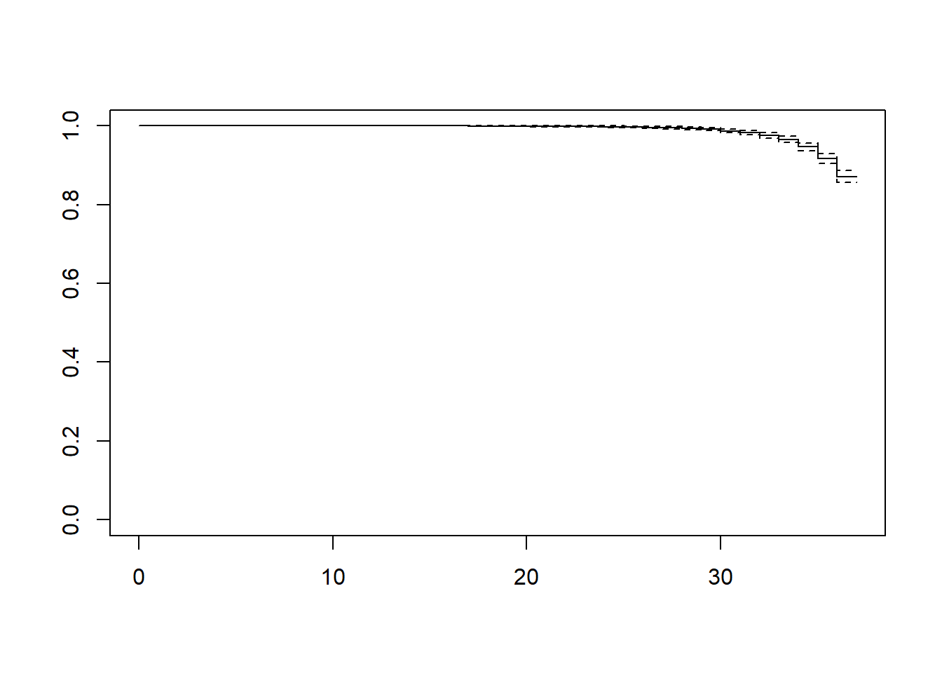
Figure 7.4: Default survival function plot
Figure 7.5 zooms in on the x- and y-axes using xlim and ylim, adds some labels, customizes the x-axis tick mark locations, and adds markings to identify censored times.
plot(surv.ex7.1, xlab = "Gestational age (weeks)", ylab = "Survival probability",
     xlim = c(16, 37), ylim = c(0.85, 1),
     mark.time = T, # Identify censored times
     xaxt = "n")    # Suppress the x-axis so we can customize it
axis(1, at = c(seq(17, 36, 3), 37)) # Customize location of tick marks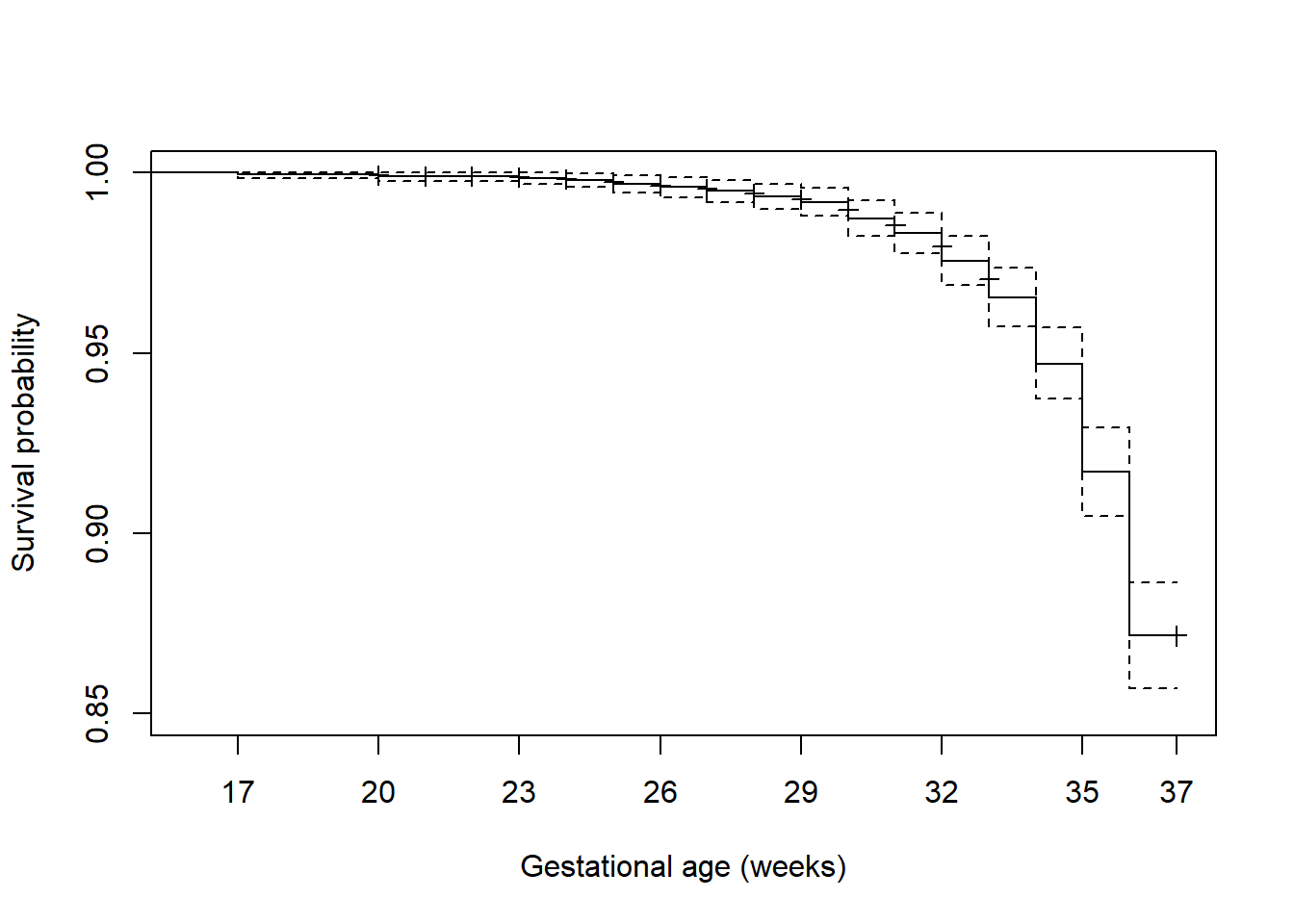
Figure 7.5: Customized survival function plot
While it is nice to have confidence bands, if they obscure the survival function they can be removed using conf.int = F (Figure 7.6).
plot(surv.ex7.1, xlab = "Gestational age (weeks)", ylab = "Survival probability",
     xlim = c(16, 37), ylim = c(0.85, 1),
     mark.time = T, # Identify censored times
     xaxt = "n",    # Suppress the x-axis so we can customize it
     conf.int = F)
axis(1, at = c(seq(17, 36, 3), 37)) # Customize location of tick marks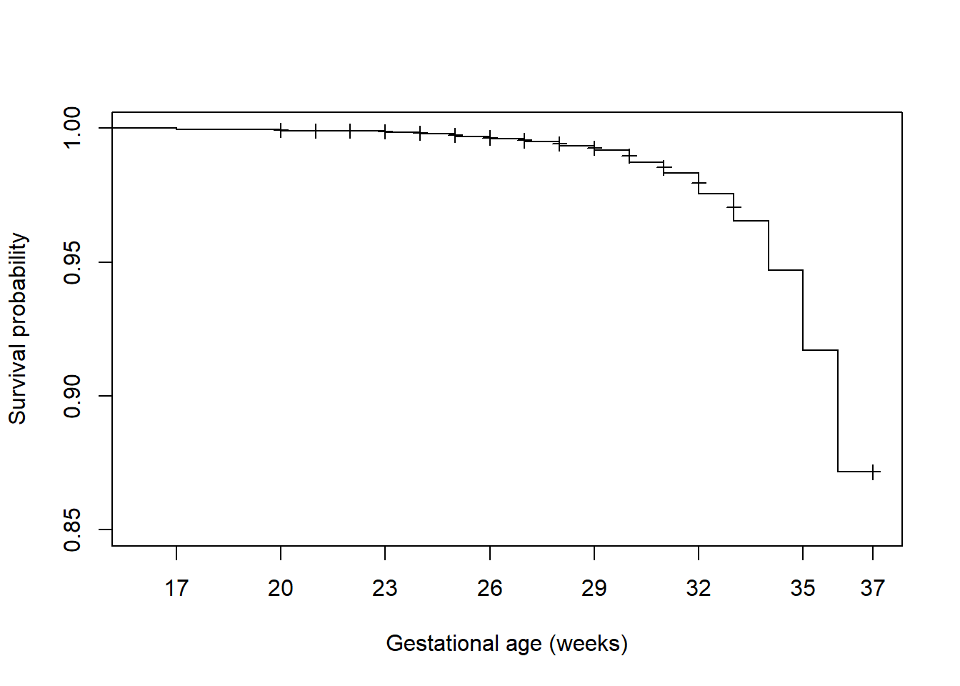
Figure 7.6: Survival function plot without confidence bands
7.6.2 Computing and plotting the hazard function
Use the bshazard() function in the bshazard library to compute the hazard function (Paola Rebora and Reilly 2024). When using bshazard, it is possible to have non-convergence leading to an error. The method uses an algorithm to smooth the estimated curve, and the nk option controls the amount of smoothing. In this case, the default value of 31 leads to an error. If there is an error, or if you just want to see what the function looks like with a different amount of smoothing, enter a different value for nk (Figure 7.7).
haz.ex7.1 <- bshazard::bshazard(Surv(gestage37, preterm01) ~ 1,
  data = natality,
  verbose = F, # Suppress display of the iteration steps
  nk=15)
plot(haz.ex7.1, conf.int = F, xlab = "Gestational age (days)",
     xlim = c(16, 37), lwd = 2, xaxt = "n")
axis(1, at = c(seq(17, 36, 3), 37))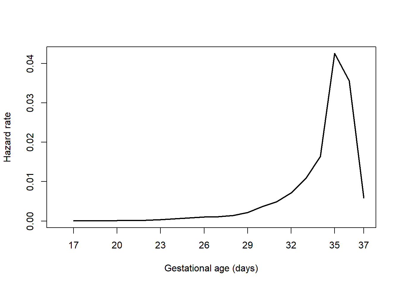
Figure 7.7: Hazard function plot
7.6.3 Estimating the event probability within a time interval
Use the KM estimate of \(S(t)\) to estimate the probability an event occurs within a specific time interval. For example, in the Natality teaching dataset, what is the estimated probability that a woman will experience a preterm birth from 33 to 35 weeks, inclusive? Be careful when figuring out how to compute this probability – the correct answer depends on whether or not we include or exclude each endpoint of the interval.
We start with the answer and then explain how it was derived.
\[P(33 \leq T \leq 35) = S(32) - S(35)\]
Why \(S(32)\) on right right-hand side instead of \(S(33)\)? Why \(S(32) - S(35)\) instead of \(S(35) - S(32)\)? \(S(35) = P(T > 35)\) is the probability of survival past 35 weeks and so is the sum of the probabilities of preterm birth occurring at 36 weeks and beyond (because the times are discrete, \(P(T > 35) = P(T \geq 36)\)). Similarly, \(S(32)\) is the sum for 33 weeks and beyond. So if we subtract these two, we are left with \(P(T = 33) + P(T = 34) + P(T = 35)\), as shown in Figure 7.8. The distance between the horizontal gray dashed lines is the sum of the drops in \(S(t)\) at weeks 33, 34, and 35.
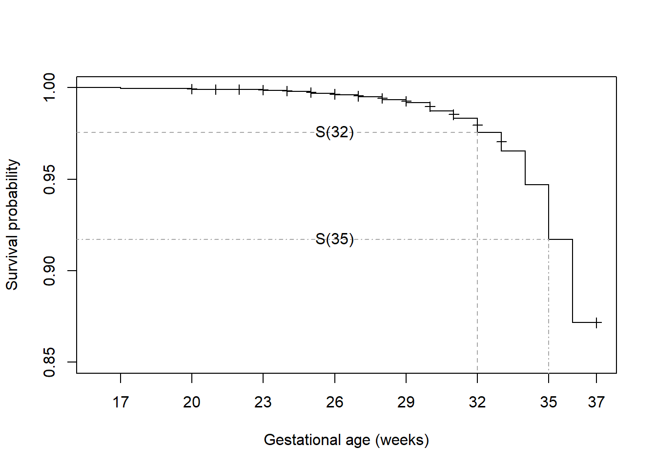
Figure 7.8: Probabiliy of an event between two times
Extract these probabilities from the summary() of the survfit object using the times option and subtract to compute \(P(33 \leq T \leq 35) = 0.0587\).
S32 <- summary(surv.ex7.1, times=32)$surv
S35 <- summary(surv.ex7.1, times=35)$surv
c(S32, S35, S32 - S35)
## [1] 0.97564 0.91697 0.05867Extracting information from a survfit object at a subset of times
The syntax summary(surv.ex7.1) produces a table showing the number at risk, number of events, and survival probability at each unique event time. We used the times option above to extract just the survival probability at a single time. More generally, you can use times to extract all the summary information at any subset of times. For example, here is the information for the first five event times.
## Call: survfit(formula = Surv(gestage37, preterm01) ~ 1, data = natality)
##
##  time n.risk n.event survival   std.err lower 95% CI upper 95% CI
##    17   2000       1   0.9995 0.0004999       0.9985       1.0000
##    20   1999       1   0.9990 0.0007068       0.9976       1.0000
##    23   1988       1   0.9985 0.0008668       0.9968       1.0000
##    24   1983       1   0.9980 0.0010020       0.9960       1.0000
##    25   1978       2   0.9970 0.0012291       0.9946       0.9994
You can also include times without events to get even more information than was obtained from summary(). For example, enter a range of times that includes times with and without events and including censored times to see how n.risk and \(S(t)\) change depending on the timing of events and censored times.
## Call: survfit(formula = Surv(gestage37, preterm01) ~ 1, data = natality)
##
##  time n.risk n.event survival   std.err lower 95% CI upper 95% CI
##    17   2000       1   0.9995 0.0004999       0.9985       1.0000
##    18   1999       0   0.9995 0.0004999       0.9985       1.0000
##    19   1999       0   0.9995 0.0004999       0.9985       1.0000
##    20   1999       1   0.9990 0.0007068       0.9976       1.0000
##    21   1997       0   0.9990 0.0007068       0.9976       1.0000
##    22   1992       0   0.9990 0.0007068       0.9976       1.0000
##    23   1988       1   0.9985 0.0008668       0.9968       1.0000
##    24   1983       1   0.9980 0.0010020       0.9960       1.0000
##    25   1978       2   0.9970 0.0012291       0.9946       0.9994
survival is constant over some of the rows, because it only changes at times with an event.
n.risk is also constant over some rows, because it only changes at times for which there was an event or censored time at the previous time. The table does not show the number of censored times, but they can be inferred by looking to see where n.risk drops by more than the previous n.event. For example, at \(t\) = 21 weeks, n.risk drops by 2 despite there being only one event at the previous time. Thus, we infer that there was one individual censored at \(t\) = 20 weeks.
When using the times option, n.event at the first time requested is the cumulative number of events up to and including that time. The table below is identical to the last three rows of the table above, except for n.event in the first row.
## Call: survfit(formula = Surv(gestage37, preterm01) ~ 1, data = natality)
##
##  time n.risk n.event survival   std.err lower 95% CI upper 95% CI
##    23   1988       3   0.9985 0.0008668       0.9968       1.0000
##    24   1983       1   0.9980 0.0010020       0.9960       1.0000
##    25   1978       2   0.9970 0.0012291       0.9946       0.9994
Similarly, if you request a single time, n.event is the cumulative number of events up to and including that time.
## Call: survfit(formula = Surv(gestage37, preterm01) ~ 1, data = natality)
##
##  time n.risk n.event survival  std.err lower 95% CI upper 95% CI
##    25   1978       6    0.997 0.001229       0.9946       0.9994
If you want to extract the number of events at a given time, you can do so by subtraction of the cumulative n.event values at the current and previous times.
## [1] 2Estimating the event probability within other time intervals
What if, instead of the probability in a two-sided interval, you want the probability of preterm birth at a specific time, prior to a certain time, or after a certain time? All the possibilities are listed below. For each, the correct computation formula depends on whether inequalities are strict or not strict.
The actual observed (non-censored) times in a dataset are finite, and you can sort them and list them in order from least to greatest. Let \(t_{\textrm{prev}}\) refer to the observed event time in the data that precedes \(t\). For example, if the data includes observed events at 5, 8, 12, and 13 days, then, for \(t = 8\), \(t_{\textrm{prev}} = 5\). If \(t\) is the earliest observed event time, then \(t_{\textrm{prev}}\) can be any number smaller than \(t\).
- \(P(t_1 \leq T \leq t_2) = S(t_{1\textrm{prev}}) - S(t_2)\)
- \(P(t_1 < T \leq t_2) = S(t_1) - S(t_2)\)
- \(P(t_1 \leq T < t_2) = S(t_{1\textrm{prev}}) - S(t_{2\textrm{prev}})\)
- \(P(t_1 < T < t_2) = S(t_1) - S(t_{2\textrm{prev}})\)
- \(P(T > t) = S(t)\)
- \(P(T \geq t) = S(t_{\textrm{prev}})\)
- \(P(T \leq t) = 1 - S(t)\)
- \(P(T < t) = 1 - S(t_{\textrm{prev}})\)
- \(P(T = t) = S(t_{\textrm{prev}}) - S(t)\)
In the Natality teaching dataset, the observed event times are
## [1] 17 20 23 24 25 26 27 28 29 30 31 32 33 34 35 36Suppose, for example, that \(t_1\) = 23 and \(t_2\) = 30. Then \(t_{1\textrm{prev}}\) = 20 and \(t_{2\textrm{prev}}\) = 29. Therefore:
- \(P(23 \leq T \leq 30) = S(20) - S(30)\)
- \(P(23 < T \leq 30) = S(23) - S(30)\)
- \(P(23 \leq T < 30) = S(20) - S(29)\)
- \(P(23 < T < 30) = S(23) - S(29)\)
- \(P(T > 23) = S(23)\)
- \(P(T \geq 23) = S(20)\)
- \(P(T \leq 23) = 1 - S(23)\)
- \(P(T < 23) = 1 - S(20)\)
- \(P(T = 23) = S(20) - S(23)\)
After computing each of the four \(S(t)\) values needed,
S20 <- summary(surv.ex7.1, times=20)$surv
S23 <- summary(surv.ex7.1, times=23)$surv
S29 <- summary(surv.ex7.1, times=29)$surv
S30 <- summary(surv.ex7.1, times=30)$surv

survprobs <- data.frame(c(20, 23, 29, 30),
                        c(S20, S23, S29, S30))
names(survprobs) <- c("t", "S(t)")
survprobs
## t S(t)
## 1 20 0.9990
## 2 23 0.9985
## 3 29 0.9919
## 4 30 0.9873Use the formulas above to derive the following:
data.frame(Interval = c("P(23 <= T <= 30)",
                        "P(23 < T <= 30)",
                        "P(23 <= T < 30)",
                        "P(23 < T < 30)",
                        "P(T > 23)",
                        "P(T >= 23)",
                        "P(T <= 23)",
                        "P(T < 23)",
                        "P(T = 23)"),
           Probability = c(S20 - S30,
                           S23 - S30,
                           S20 - S29,
                           S23 - S29,
                           S23,
                           S20,
                           1 - S23,
                           1 - S20,
                           S20 - S23))
## Interval Probability
## 1 P(23 <= T <= 30) 0.0116579
## 2 P(23 < T <= 30) 0.0111553
## 3 P(23 <= T < 30) 0.0070845
## 4 P(23 < T < 30) 0.0065820
## 5 P(T > 23) 0.9984975
## 6 P(T >= 23) 0.9990000
## 7 P(T <= 23) 0.0015025
## 8 P(T < 23) 0.0010000
## 9 P(T = 23) 0.00050257.6.4 Median survival time
The median survival time is the time at which 50% of the individuals have experienced the event and 50% have not. On the survival function, \(S(\textrm{median survival time})\) = 0.50. In Example 7.1, the probability of “survival” (not having a preterm birth) never dropped below 0.8716 so the median survival time is not defined. Look at an example for which the probability does go below 0.50.
Example 7.3: The teaching dataset based on the Framingham Heart Study (see Appendix A.6) contains information about whether or not participants experienced hypertension (HYPERTEN) and how long (in days) after baseline until they were diagnosed as hypertensive (TIMEHYP). If there were no censoring, we could simply compute the median of the event times to compute the median survival time. We must include na.rm = T as individuals with prevalent hypertension at baseline have missing values for TIMEHYPE and HYPERTEN, so analyses of this variable are restricted to individuals who were not hypertensive at baseline.
## [1] 5094The median of the event time variable is 5094.5. However, some of the event times are censored (some values of HYPERTEN, the event indicator, are 0) so the raw median is an underestimate – it treats censored times as event times when in fact the individual’s actual time of diagnosis, if they ever were diagnosed, is later. Use survfit() to view the median survival time accounting for censoring, and its 95% confidence interval.
## Call: survfit(formula = Surv(TIMEHYP, HYPERTEN) ~ 1, data = fram_time_invar)
##
##    1299 observations deleted due to missingness
##         n events median 0.95LCL 0.95UCL
## [1,] 2916   1767   5837    5620    6069
To extract the median and confidence interval, use summary() on the survfit object.
##  median 0.95LCL 0.95UCL
##    5837    5620    6069
For this example, the time is in days, so divide by 365.25 to get the median survival time in years.
##  median 0.95LCL 0.95UCL
##   15.98   15.39   16.62
The median survival time is 5837 days, or 15.98 years (95% CI = 15.39, 16.62). Since \(P(T > \textrm{median}) = 0.50\), we know that \(P(T \leq \textrm{median}) = 0.50\), so the median survival time (time still free of hypertension) is also the median time of diagnosis.
On the survival function, the median time is the time at which the curve crosses 0.50 (Figure 7.9).
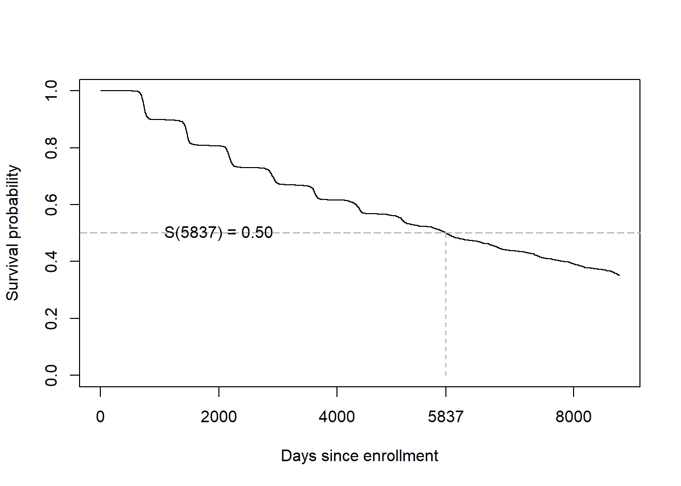
Figure 7.9: Median survival time
7.6.5 Comparing groups
So far we have only used the KM estimator to compute the overall survival function for all individuals in the dataset pooled together regardless of how their characteristics differ. We can also estimate separate curves for groups with different characteristics and use the log-rank test to test the null hypothesis that the groups’ survival functions are the same. In the model formula, place the grouping variable on the right-hand side. Use survfit() to facilitate plotting, and survdiff() (Harrington and Fleming 1982) to carry out the log-rank test.
Example 7.4: In the United States, there are large racial disparities in the risk of preterm birth, with Black women having much greater risk than White women (Burris et al. 2019). Compare the time to preterm birth between mothers of different race/ethnicity (MRACEHISP) in the Natality teaching dataset.
First, compute the KM estimate of survival.
## Call: survfit(formula = Surv(gestage37, preterm01) ~ MRACEHISP, data = natality)
##
##    9 observations deleted due to missingness
##                       n events median 0.95LCL 0.95UCL
## MRACEHISP=NH White 1028    100     NA      NA      NA
## MRACEHISP=NH Black  300     62     NA      NA      NA
## MRACEHISP=NH Other  188     20     NA      NA      NA
## MRACEHISP=Hispanic  475     69     NA      NA      NA
The median event times are all NA, since the proportion of preterm births is always above 0.50 in every group. Figure 7.10 illustrates the survival functions. plot() automatically creates separate lines for each group. The previous output shows that there are four groups, so there are four survival functions. The lty = 1:4 option in plot() provides a distinct line type for each group. Note how c(1,3,4,2) was used to change the ordering of lty and the group labels in legend() so the legend order matches the order of the lines in the plot.
plot(surv.ex7.4,
  xlab = "Gestational age (weeks)", ylab = "Survival probability",
  xlim = c(17, 37), ylim = c(0.75, 1),
  conf.int = F, mark.time = F,
  lty = 1:4) # 4 groups
# Add c(1,3,4,2) in two places to re-order the legend to match
# the ordering of the lines at 37 weeks
legend(20, 0.95,
  # Inside c(), the ordering is the same as the order shown in surv.ex7.4
  levels(natality$MRACEHISP)[c(1,3,4,2)],
  lty = c(1,3,4,2),
  title = "Mother's Race/Ethnicity")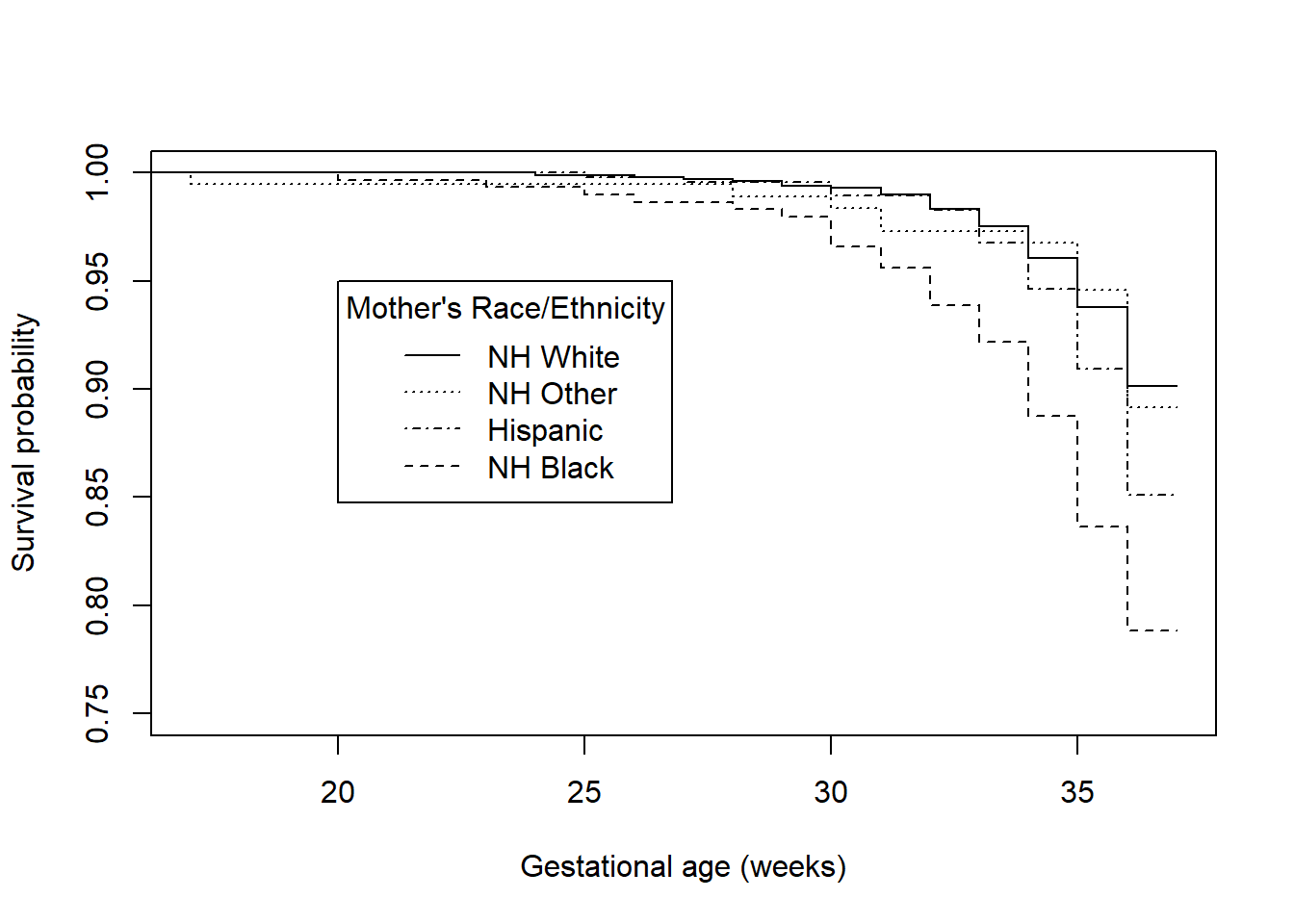
Figure 7.10: Survival functions for time to preterm birth by race/ethnicity
Similarly, plot() automatically plots a separate hazard function for each group (Figure 7.11).
# In this case, the default amount of smoothing does not lead to
# an error, so we do not need to specify nk unless we want to
# see what it looks like with less smoothing
haz.ex7.4 <- bshazard::bshazard(Surv(gestage37, preterm01) ~ MRACEHISP,
     data = natality,
     verbose = F)
## NOTE: entry.status has been set to 0 for all.plot(haz.ex7.4,
xlab = "Gestational age (weeks)",
ylab = "Hazard of preterm birth",
conf.int = F, overall = F,
lty = 1:4, ylim = c(0, 0.08))
legend(10, 0.05,
levels(natality$MRACEHISP)[c(2,4,3,1)],
lty = c(2,4,3,1), title = "Mother's Race/Ethnicity")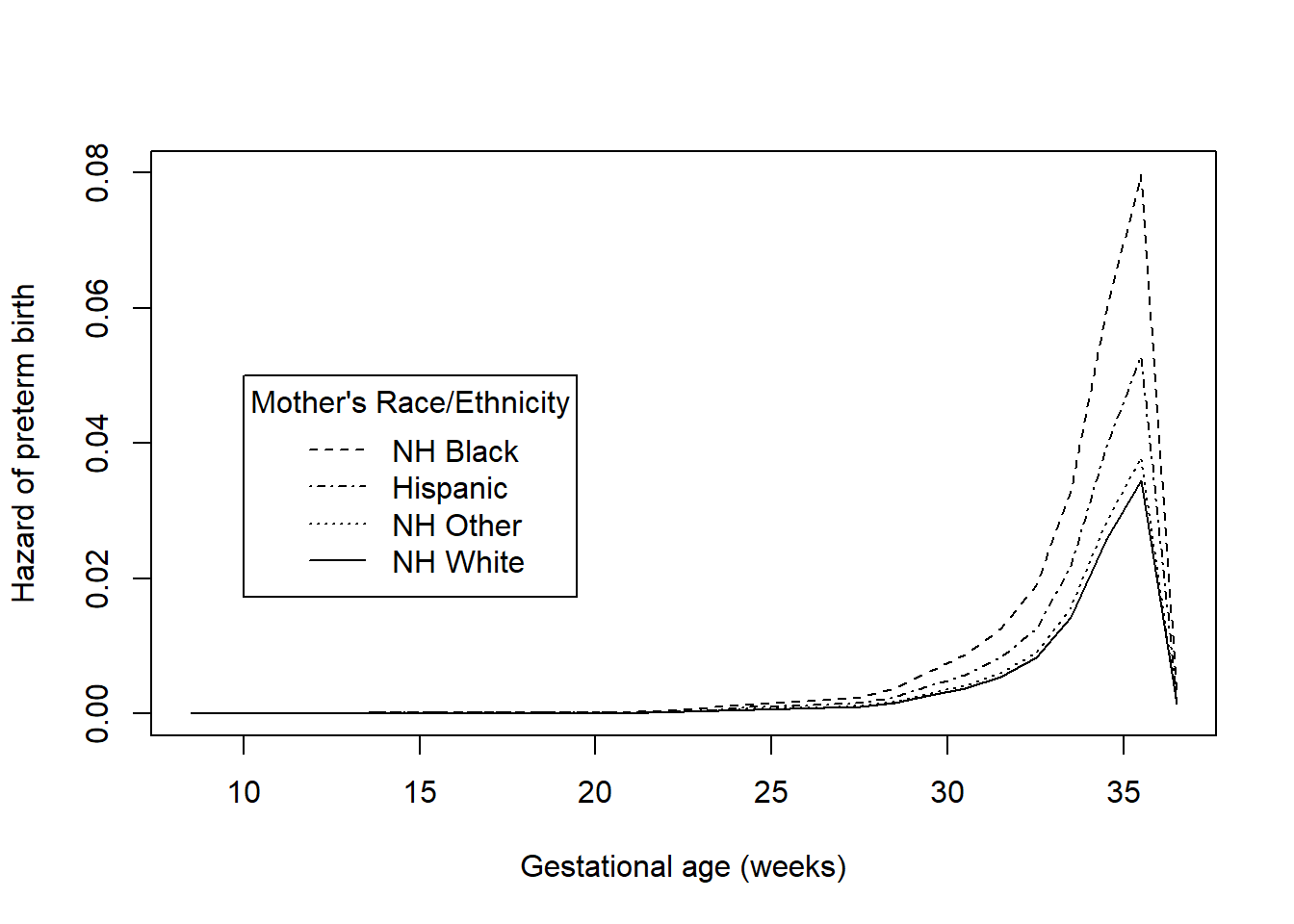
Figure 7.11: Hazard functions for time to preterm birth by race/ethnicity
Finally, use survdiff() to carry out the log-rank test comparing the groups.
## Call:
## survdiff(formula = Surv(gestage37, preterm01) ~ MRACEHISP, data = natality)
##
## n=1991, 9 observations deleted due to missingness.
##
##                       N Observed Expected (O-E)^2/E (O-E)^2/V
## MRACEHISP=NH White 1028      100    132.0     7.778    16.897
## MRACEHISP=NH Black  300       62     35.4    19.969    23.927
## MRACEHISP=NH Other  188       20     24.0     0.678     0.772
## MRACEHISP=Hispanic  475       69     59.5     1.515     2.044
##
##  Chisq= 30.8  on 3 degrees of freedom, p= 0.0000009
Unfortunately, the p-value is not one of the numbers you can extract directly from the survdiff object. However, you can compute it directly using pchisq(, lower.tail=F) by extracting the chisq value and computing the degrees of freedom as one less than the number of levels.
## [1] 0.0000009284The racial disparity in preterm birth can be seen in both the survival and hazard function plots – Hispanic and non-Hispanic Black mothers have lower survival (non-preterm birth) probabilities and greater hazards than non-Hispanic White and non-Hispanic Other race mothers. Based on the log-rank test, this difference is statistically significant (\(\chi^2 = 30.8\), df = 3, p <.001). In Section 7.7 we will estimate the magnitude of the ratio of the hazards between each pair of race/ethnicity values. While the log-rank test is useful as a hypothesis test, it does not provide an estimate of effect size.