10.7 Optional: Two-way tables
Applying tattoos carries health risks as the skin is broken during application. An American study examined if a relationship existed between having hepatitis C and having tattoos (Haley and Fischer 2001).
To study this, \(626\) people were interviewed as part of an observational study, and asked about two issues: Whether they had hepatitis C (\(47\) people) or not (\(579\) people); and if they had a tattoo (\(113\) people), or no tattoos (\(513\) people).
Which one of these five sets of hypotheses is not valid for this situation? Why?
- \(H_0\): No association between having hepatitis C and having a tattoo in the population;
\(H_1\): An association between having hepatitis C and having a tattoo in the population. - \(H_0\): The odds of having hepatitis C is the same with or without a tattoo in the population;
\(H_1\): The odds of having hepatitis C is not the same with or without a tattoo in the population. - \(H_0\): The mean number of people having hepatitis C is the same for those with and without a tattoo in the population;
\(H_1\): The mean number of people having hepatitis C is not the same for those with and without a tattoo in the population. - \(H_0\): The odds ratio of having hepatitis C, comparing those with or without a tattoo, is one in the population;
\(H_1\): The odds ratio of having hepatitis C, comparing those with or without a tattoo, is not one in the population. - \(H_0\): The proportion having hepatitis C is the same with or without a tattoo in the population;
\(H_1\): The proportion having hepatitis C is not the same with or without a tattoo in the population.
- \(H_0\): No association between having hepatitis C and having a tattoo in the population;
Compute the percentage of people overall in the sample with a tattoo.
Assuming the null hypothesis about the population is true, compute the number of people in the sample with hepatitis C that you would expect have a tattoo. Use the information above to answer the question.
In the sample, \(25\) people had Hep. C and a tattoo. Use this information to create the two-way table summarising the data (Table 10.3).
| Had Hep. C | Did not have Hep. C | Total | |
|---|---|---|---|
| Had tattoo | |||
| Did not have tattoo | |||
| Total | 626 |
- In the sample, what are the odds that someone has Hep. C, among those with a tattoo?
- In the sample, what are the odds that someone has Hep. C, among those without a tattoo?
- From the sample information, compute the odds ratio of having Hep. C, comparing students with a tattoo to those without a tattoo. Carefully explain what this value means.
10.7.1 Optional: Comparing two independent means
A study compared the number of deaths reported from hurricanes with male and female names (Smith 2016). One of the tables in the paper is shown in Fig. 10.6. Explain in everyday language what this means.
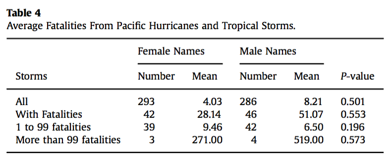
FIGURE 10.6: Table 4 from Smith (2016)
10.7.3 Optional: Tests for comparing the mean from two independent samples
(Answers available in Sect. A.10)
This question is optional; e.g., if you need more practice, or you are studying for the exam.
This question has a video solution in the online book, so you can hear and see the solution.
Batteries are expensive, so comparing the performance of expensive and cheap batteries is helpful.
A test on the lifetime of batteries (Lindström 2011) compared the time for two brands of \(1.5\) volt batteries to reduce their voltage to \(1.0\) volts under standard testing conditions.
The times (in hours) for nine Energizer Max batteries and nine ALDI brand batteries (Ultracell) are shown in Table 10.4.
| Energizer | 7.58 | 7.46 | 7.46 | 7.59 | 7.46 | 7.52 | 6.83 | 6.89 | 7.45 |
| Ultracell | 7.5 | 7.48 | 7.47 | 7.48 | 7.48 | 7.41 | 7.47 | 6.96 | 7.48 |
Write the hypotheses for testing the research question of interest. Is the test one- or two-tailed?
Explain the meaning of the standard error of the mean in this context.
The software output for the analysis is shown in Fig. 10.7 (jamovi) and Fig. 10.8 (SPSS). Determine the value of the \(t\)-statistic and the \(P\)-value for testing the hypotheses.
Write a statement that communicates the result of the test.
What conditions must be met for this test to be valid?
Is it reasonable to assume the assumptions are satisfied?
What did you learn from this study?
At the time of this analysis, a four-pack of the Ultracell Max batteries cost $2.49 from ALDI online, while a four pack of Energizer Max from Woolworths online cost $5.97 on special (usually $8.01)3.
On the basis of this information, would you be prepared to try the Ultracell batteries? Explain your reasoning.
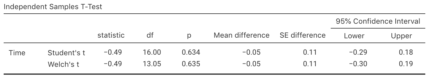
FIGURE 10.7: Output from jamovi for the battery data
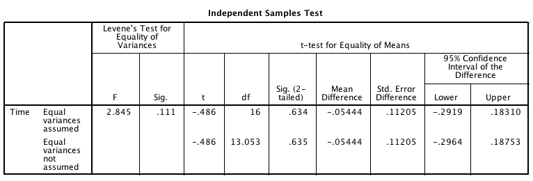
FIGURE 10.8: Output from SPSS for the battery data
10.7.4 Optional: Tests for ORs
A study (Higgins and Koch 1977) studied byssinosis (a respiratory complaint) among workers in the textile industry. The researchers were interested, among other things, in exploring the relationship between smoking status and the presence of byssinosis.
More specifically, they wanted to see if the proportion of smokers with byssinosis was greater than the proportion of non-smokers with byssinosis, among all textile workers.
The researchers used an observational study.
Which one of these is correct as a null hypothesis? Why are the others incorrect?
- The odds of having byssinosis is the same in the sample of smokers and the sample of non-smokers.
- The mean number of workers having byssinosis is the same for smokers and non-smokers.
- The population odds of having byssinosis is the same in among smokers and non-smokers.
Among those randomly selected to appear in the study, \(165\) workers had byssinosis (\(40\) were non-smokers) and \(5254\) did not (\(2190\) were non-smokers).
Construct the two-way table showing the number of workers with byssinosis among smokers and non-smokers.
Compute the sample proportion of workers with byssinosis, among smokers. Then, compute the sample proportion of workers with byssinosis, among non-smokers.
Compute the odds of having byssinosis, among smokers. Then compute the odds of having byssinosis, among non-smokers. What do these odds mean?
Compute the odds ratio comparing smokers to non-smokers. What does this odds ratio mean?
A report states that the odds ratio is not one simply due to sampling variation, and not due to smoking.
Do you agree or disagree? Why?Use the software output in Fig. 10.9 (jamovi) or Fig. 10.10 and Fig. 10.11 (SPSS), to test the hypotheses. Write a proper conclusion to communicate the results.
Are the results likely to be statistically valid? Explain.
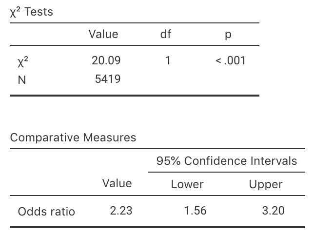
FIGURE 10.9: Output from jamovi for the byssinosis example
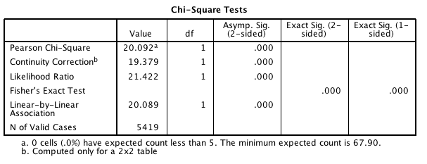
FIGURE 10.10: Output from SPSS for the byssinosis example
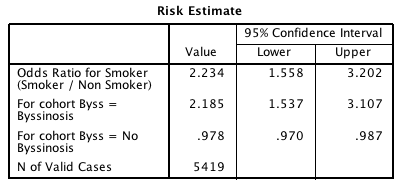
FIGURE 10.11: More output from SPSS for the byssinosis example
10.7.5 Optional: Tests for ORs
This question has a video solution in the online book, so you can hear and see the solution.
A study (Tanagawa and Shigematsu 1998) examined the choice of airway devices used for nontraumatic, out-of-hospital cardiac arrest patients, to evaluate the success and failure of insertion for various devices.
The data for success and failure at insertion is given in Table 10.5, taken from available patient documentation.
| Succeed | Fail | |
|---|---|---|
| Esophageal gastric tube airway (EGTA) | 545 | 49 |
| Laryngeal mask (LM) | 2701 | 315 |
Define \(p\) as the population proportion of successful attempts at insertion. Write the hypotheses to be tested.
Use the software output in Fig. 10.12 (jamovi) or Fig. 10.13 (SPSS) to test the hypotheses. Write a proper conclusion to communicate the results.
Are the results likely to be statistically valid? Explain.
The study was designed to enable medics to choose the best airway device.
Would you recommend EGTA or LM? Why? Would you like any more information before making your choice? Explain.

FIGURE 10.12: The jamovi output for the table from Tanagawa and Shigematsu (1998)
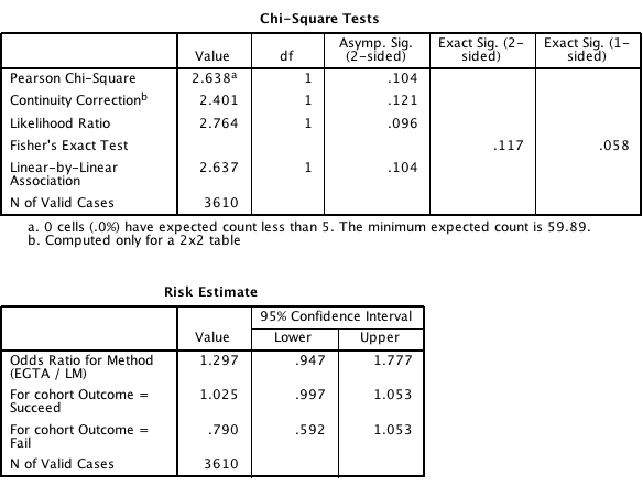
FIGURE 10.13: The SPSS output for the table from Tanagawa and Shigematsu (1998)
References
Data from 05 September 2012.↩︎