7.7 Optional questions
These questions are optional; e.g., if you need more practice, or you are studying for the exam. (Answers appear in Sect. A.7.)
7.7.2 (Optional) CI for one mean
This question has a video solution in the online book, so you can hear and see the solution.
Shortly after metric units were introduced to Australia in 1977, a lecturer wondered how accurately students could estimate lengths using the metric measurements (Hand et al. 1996).
The aim of the study was to determine if, on average, students could correctly guess the width of the hall (which was \(13.1\,\text{m}\)).
To answer the RQ, a group of \(n = 44\) students were asked to estimate the width of the lecture hall to the nearest metre (data provided by Prof. Lewis). The data are given in Table 7.1.
The data were entered into software, producing the output in Fig. 7.5 (jamovi).
| 8 | 9 | 10 | 10 | 10 | 10 | 10 | 10 | 11 | 11 | 11 | 11 | 12 | 12 | 13 |
| 13 | 13 | 14 | 14 | 14 | 15 | 15 | 15 | 15 | 15 | 15 | 15 | 15 | 16 | 16 |
| 16 | 17 | 17 | 17 | 17 | 18 | 18 | 20 | 22 | 25 | 27 | 35 | 38 | 40 |
- What is the value of \(\bar{x}\)?
- What are the values of \(s\) and \(\text{s.e.}(\bar{x})\)? Explain the difference in the meaning of the two terms.
- Write down the \(95\)% CI for the population estimate (see Fig. 7.5 (jamovi).
- What conditions must be met for this test to be statistically valid?
- Is it reasonable to assume the statistical validity conditions are satisfied? How does the histogram in Fig. 7.4 help, if at all?
- Do you think students were very good at estimating the width of the hall using metric units? Explain.
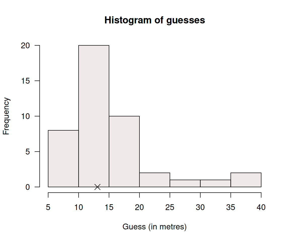
FIGURE 7.4: Histogram for the estimates of the width of a hall by \(n = 44\) students. The cross is the actual width of the hall.
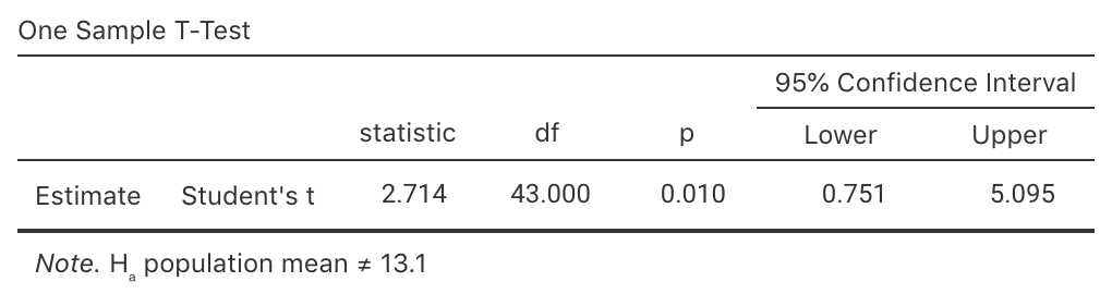
FIGURE 7.5: jamovi output for the estimates of the width of a hall in metres
7.7.3 (Optional) CI for one proportion
This question has a video solution in the online book, so you can hear and see the solution.
The timing of pubertal maturation can vary, which can have impacts upon behaviour. Duncan et al. (1985) studied (p. 231):
...the relationships between maturational timing and body image, school behavior, and deviance
Sample data were collected from
...children and youth of the entire United States drawn by the National Center for Health Statistics... known as the National Health Examination Survey (1966--1970). Data were collected on \(5\,735\) adolescents' physical and psychological status...
- What type of research question is being answered: descriptive, relational, repeated-measures or correlational? Explain.
- For the \(2\,864\) males in the sample, \(352\) were classified as maturing late. Compute the sample estimate of the population proportion of males who mature late.
- Compute the precision of this estimate (that is, the standard error).
- Compute an approximate \(95\)% confidence interval for the population proportion of boys that mature late based on the sample proportion.
- Confirm that the conditions necessary for this calculation to be statistically valid are met.
- If the researchers wished to estimate the true proportion of boys that mature late to within give-or-take \(0.02\) with \(95\)% confidence, would a larger or smaller sample be needed? Explain.