9.6 Optional questions
These questions are optional; e.g., if you need more practice, or you are studying for the exam. (Answers appear in Sect. A.9.)
9.6.1 (Optional) Paired \(t\)-test
Hébert-Losier et al. (2023) recorded double-legged jumping distance for \(80\) healthy people, when they wore shoes and were barefoot. The data are too large to show here, but use the jamovi output (Fig. 9.8) to answer the following questions.
- What do the differences mean (as given in the output)?
- Create a numerical summary table for the data.
- Determine \(95\)% CI for the difference in height of the two jumps.
- Conduct a hypothesis test to determine if a mean difference exists in the population.
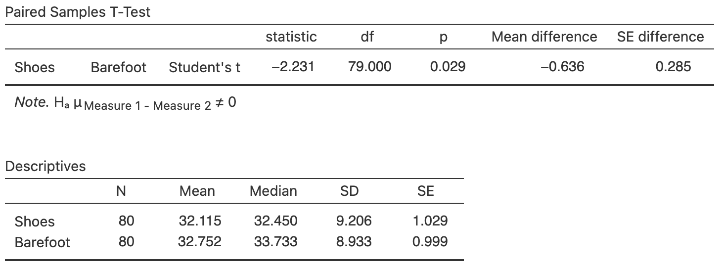
FIGURE 9.8: The jamovi output summarising the jumping data.
9.6.2 (Optional) Two-sample \(t\)-test
Strayer and Johnston (2001) examined the reaction times, while driving, for students from the University of Utah (Agresti and Franklin 2007). In one study, students were randomly allocated to one of two groups:
- one group used a mobile phone while driving in a driving simulator; and
- one group did not use a mobile phone while driving in a driving simulator.
The reaction time for each student was measured. The data are shown below. Use the information in Table 9.2 to answer this RQ:
For students, is there a difference between the mean reaction time while driving when using a mobile phone and when not using a mobile phone?
Be sure to include an approximate \(95\)% CI as well as the hypothesis test results.
| Mean | Sample size | Std dev. | Std error | |
|---|---|---|---|---|
| Using phone | \(533.59\) | \(32\) | \(65.36\) | \(11.554\) |
| Not using phone | \(585.19\) | \(32\) | \(89.65\) | \(15.847\) |
| Differences | \(\phantom{0}51.59\) | \(19.612\) |