11.3 Interpreting regressions

I was wondering about how the age of second-hand cars impact their price. On 25 June, 2014, I searched Gum Tree, for Toyota Corolla in the 'Cars, Vans & Utes' category. The age and the price of each (second-hand) car was recorded from the first two pages of results that were returned.

I then restricted the data to cars $15$ years old or younger (and removed one $13$-year-old Corolla advertised for sale for $390,000, assuming this was an error). I then produced the scatterplot in Fig. 11.2.

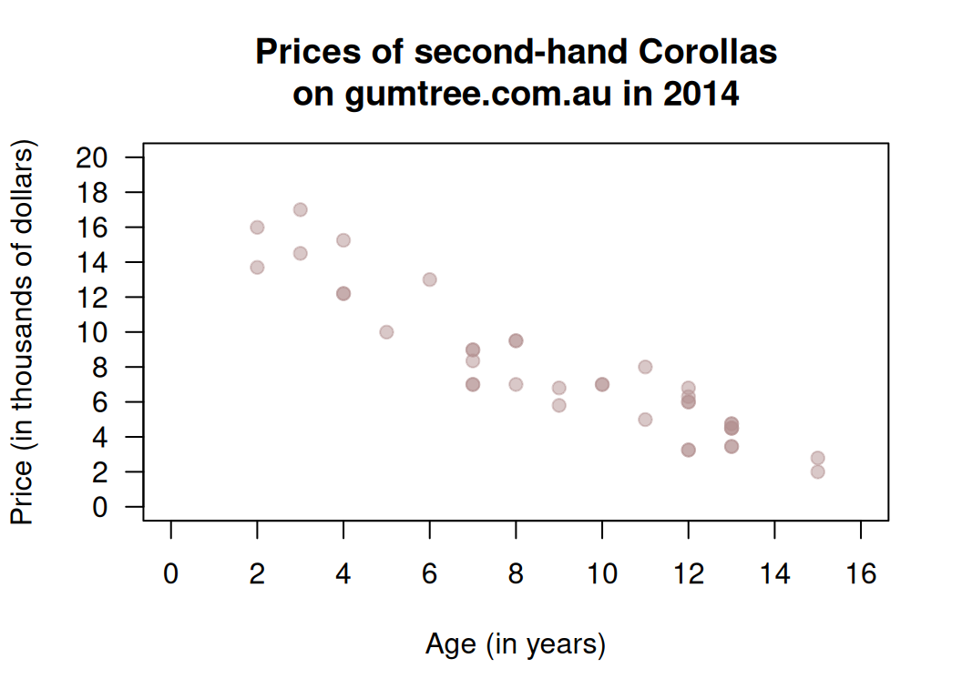
FIGURE 11.2: The price of second-hand Toyota Corollas as advertised on Gum Tree on 25 June 2014 plotted against age ($n = 38$).

Describe the relationship displayed in the graph in words.
What else could influence the price of a second-hand Corollas?
From the scatterplot, draw (if you can) or estimate by eye an approximation of the regression line.
On the scatterplot, locate a seven-year-old Corolla selling for $15,000. Would this be cheap or expensive?
As stated, I removed one observation: a $13$-year-old Corolla for sale at $390,000. What do you think the price was meant to be listed as, by looking at the scatterplot? Explain.
Estimate the value of $b_0$ (the intercept) from the line you drew. What does this mean? Do you think this value is meaningful?
Estimate the value of $b_1$ (the slope) from the line you drew. What does this mean? Do you think this value is meaningful?
From the line you drew above, write down an estimate of the regression equation.
Use the software output (Fig. 11.3 and Fig. 11.4 (jamovi)) relating the price (in thousands of dollars) to age to write down the regression equation.
Using the software output, write down the value of $r$. Using this value of $r$, compute the value of $R^2$. What does this mean?
Use the regression equation from the software output to estimate the sale price of a Corolla that is $20$ years old, and explain your answer.
Using the software output, perform a suitable hypothesis test to determine if there is evidence that lower prices are associated with older Corollas.
Compute an approximate $95$% confidence interval for the population slope (use the software output in Fig. 11.4).
I could have drawn a scatterplot with Price on the vertical (up-and-down) axis and Year of manufacture on the horizontal (left-to-right) axis (Fig. 11.5). For this graph:
1. What is the value of the correlation coefficient?
2. How would the value of $R^2$ change?
3. How would the value of the slope change?
4. How would the value of the intercept change?

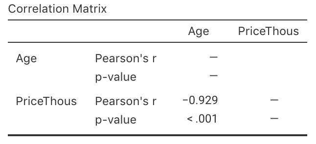
FIGURE 11.3: The jamovi correlation output, analysing the Corolla data.

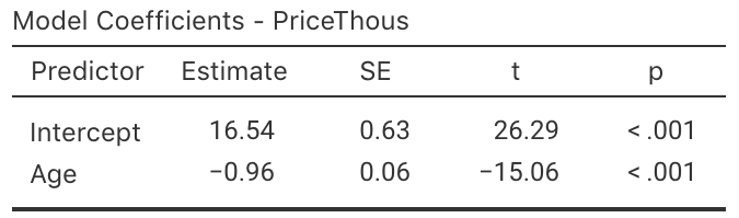
FIGURE 11.4: The jamovi regression output, analysing the Corolla data.

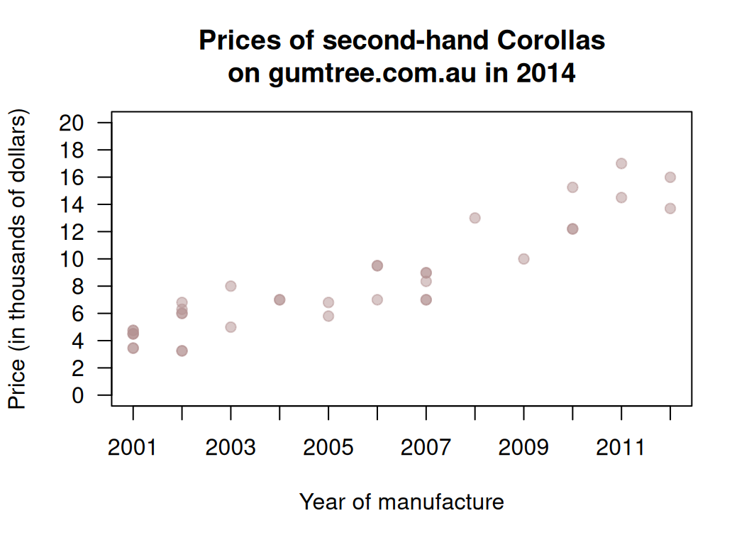
FIGURE 11.5: The price of second-hand Toyota Corollas as advertised on Gum Tree on 25 June 2014 plotted against the year of manufacture ($n=38$).