2.2 The four RStudio Windows

When you open RStudio, you’ll see the following four windows (also called panes) shown in in Figure 1.7. However, your windows might be in a different order that those in Figure 1.7. If you’d like, you can change the order of the windows under RStudio preferences. You can also change their shape by either clicking the minimize or maximize buttons on the top right of each panel, or by clicking and dragging the middle of the borders of the windows.

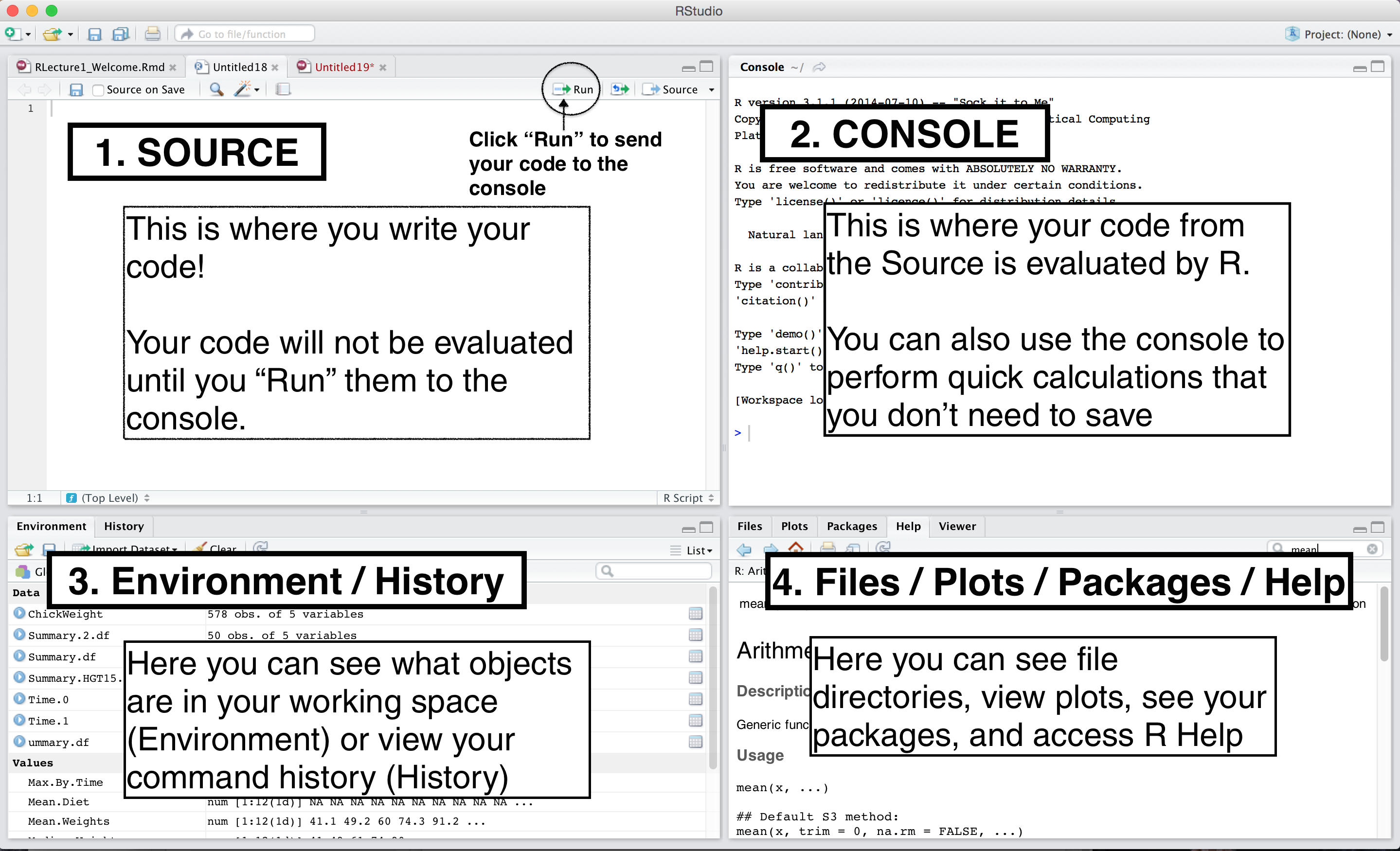
Figure 1.7: The four panes of RStudio.

Now, let’s see what each window does in detail.

2.2.1 Source - Your notepad for code

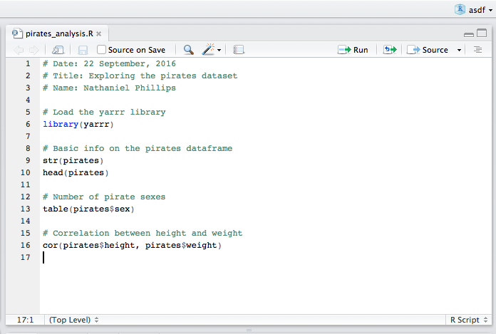
Figure 1.8: The Source contains all of your individual R scripts. The code won’t be evaluated until you send it to the Console.

The source pane is where you create and edit ``R Scripts" - your collections of code. Don’t worry, R scripts are just text files with the “.R” extension. When you open RStudio, it will automatically start a new Untitled script. Before you start typing in an untitled R script, you should always save the file under a new file name (like, “2015PirateSurvey.R”). That way, if something on your computer crashes while you’re working, R will have your code waiting for you when you re-open RStudio.

You’ll notice that when you’re typing code in a script in the Source panel, R won’t actually evaluate the code as you type. To have R actually evaluate your code, you need to first ‘send’ the code to the Console (we’ll talk about this in the next section).

There are many ways to send your code from the Source to the console. The slowest way is to copy and paste. A faster way is to highlight the code you wish to evaluate and clicking on the “Run” button on the top right of the Source. Alternatively, you can use the hot-key “Command + Return” on Mac, or “Control + Enter” on PC to send all highlighted code to the console.

2.2.2 Console: R’s Heart

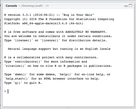
Figure 1.9: The console the calculation heart of R. All of your code will (eventually) go through here.

The console is the heart of R. Here is where R actually evaluates code. At the beginning of the console you’ll see the character . This is a prompt that tells you that R is ready for new code. You can type code directly into the console after the prompt and get an immediate response. For example, if you type 1+1 into the console and press enter, you’ll see that R immediately gives an output of 2.

1+1
## [1] 2

Try calculating 1+1 by typing the code directly into the console - then press Enter. You should see the result [1] 2. Don’t worry about the [1] for now, we’ll get to that later. For now, we’re happy if we just see the 2. Then, type the same code into the Source, and then send the code to the Console by highlighting the code and clicking the ``Run" button on the top right hand corner of the Source window. Alternatively, you can use the hot-key “Command + Return” on Mac or “Control + Enter” on Windows.

Tip: Try to write most of your code in a document in the Source. Only type directly into the Console to de-bug or do quick analyses.

So as you can see, you can execute code either by running it from the Source or by typing it directly into the Console. However, 99% most of the time, you should be using the Source rather than the Console. The reason for this is straightforward: If you type code into the console, it won’t be saved (though you can look back on your command History). And if you make a mistake in typing code into the console, you’d have to re-type everything all over again. Instead, it’s better to write all your code in the Source. When you are ready to execute some code, you can then send “Run” it to the console.

2.2.3 Environment / History

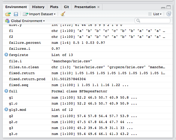
Figure 1.10: The environment panel shows you all the objects you have defined in your current workspace. You’ll learn more about workspaces in Chapter 7.

The Environment tab of this panel shows you the names of all the data objects (like vectors, matrices, and dataframes) that you’ve defined in your current R session. You can also see information like the number of observations and rows in data objects. The tab also has a few clickable actions like ``Import Dataset" which will open a graphical user interface (GUI) for important data into R. However, I almost never look at this menu.

The History tab of this panel simply shows you a history of all the code you’ve previously evaluated in the Console. To be honest, I never look at this. In fact, I didn’t realize it was even there until I started writing this tutorial.

As you get more comfortable with R, you might find the Environment / History panel useful. But for now you can just ignore it. If you want to declutter your screen, you can even just minimize the window by clicking the minimize button on the top right of the panel.

2.2.4 Files / Plots / Packages / Help

The Files / Plots / Packages / Help panel shows you lots of helpful information. Let’s go through each tab in detail:

1. Files - The files panel gives you access to the file directory on your hard drive. One nice feature of the “Files” panel is that you can use it to set your working directory - once you navigate to a folder you want to read and save files to, click “More” and then “Set As Working Directory.” We’ll talk about working directories in more detail soon.

2. Plots - The Plots panel (no big surprise), shows all your plots. There are buttons for opening the plot in a separate window and exporting the plot as a pdf or jpeg (though you can also do this with code using the pdf() or jpeg() functions.)

Let’s see how plots are displayed in the Plots panel. Run the code on the right to display a histogram of the weights of chickens stored in the ChickWeight dataset. When you do, you should see a plot similar to the one in Figure 1.11 show up in the Plots panel.

hist(x = ChickWeight$weight,
     main = "Chicken Weights",
     xlab = "Weight",
     col = "skyblue",
     border = "white")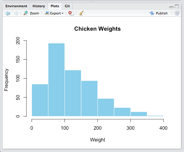

Figure 1.11: The plot panel contains all of your plots, like this histogram of the distribution of chicken weights.

3. Packages - Shows a list of all the R packages installed on your harddrive and indicates whether or not they are currently loaded. Packages that are loaded in the current session are checked while those that are installed but not yet loaded are unchecked. We’ll discuss packages in more detail in the next section.

4. Help - Help menu for R functions. You can either type the name of a function in the search window, or use the code to search for a function with the name

?hist   # How does the histogram function work?
?t.test # What about a t-test?