13.3 T-test: t.test()
To compare the mean of 1 group to a specific value, or to compare the means of 2 groups, you do a t-test. The t-test function in R is t.test(). The t.test() function can take several arguments, here I’ll emphasize a few of them. To see them all, check the help menu for t.test (?t.test).
13.3.1 1-sample t-test
| Argument | Description |
|---|---|
x |
A vector of data whose mean you want to compare to the null hypothesis mu |
mu |
The population mean under the null hypothesis. For example, mu = 0 will test the null hypothesis that the true population mean is 0. |
alternative |
A string specifying the alternative hypothesis. Can be "two.sided" indicating a two-tailed test, or "greater" or “less" for a one-tailed test. |
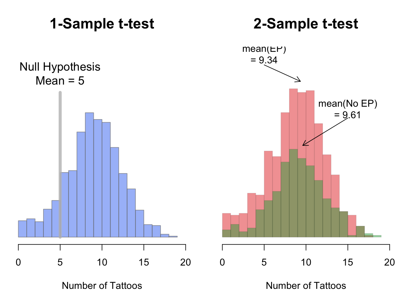
In a one-sample t-test, you compare the data from one group of data to some hypothesized mean. For example, if someone said that pirates on average have 5 tattoos, we could conduct a one-sample test comparing the data from a sample of pirates to a hypothesized mean of 5. To conduct a one-sample t-test in R using t.test(), enter a vector as the main argument x, and the null hypothesis as the argument mu
Here, I’ll conduct a t-test to see if the average number of tattoos owned by pirates is different from 5:
tattoo.ttest <- t.test(x = pirates$tattoos,  # Vector of data
                       mu = 5)               # Null: Mean is 5

# Print the result
tattoo.ttest
##
##  One Sample t-test
##
## data:  pirates$tattoos
## t = 40, df = 1000, p-value <2e-16
## alternative hypothesis: true mean is not equal to 5
## 95 percent confidence interval:
##  9.2 9.6
## sample estimates:
## mean of x
##       9.4
As you can see, the function printed lots of information: the sample mean was 9.43, the test statistic (41.59), and the p-value was 2e-16 (which is virtually 0). Because 2e-16 is less than 0.05, we would reject the null hypothesis that the true mean is equal to 5.
Now, what happens if I change the null hypothesis to a mean of 9.4? Because the sample mean was 9.43, quite close to 9.4, the test statistic should decrease, and the p-value should increase:
tattoo.ttest <- t.test(x = pirates$tattoos,
                       mu = 9.5)  # Null: Mean is 9.4

tattoo.ttest
##
##  One Sample t-test
##
## data:  pirates$tattoos
## t = -0.7, df = 1000, p-value = 0.5
## alternative hypothesis: true mean is not equal to 9.5
## 95 percent confidence interval:
##  9.2 9.6
## sample estimates:
## mean of x
##       9.4
Just as we predicted! The test statistic decreased to just -0.67, and the p-value increased to 0.51. In other words, our sample mean of 9.43 is reasonably consistent with the hypothesis that the true population mean is 9.50.
13.3.2 2-sample t-test
In a two-sample t-test, you compare the means of two groups of data and test whether or not they are the same. We can specify two-sample t-tests in one of two ways. If the dependent and independent variables are in a dataframe, you can use the formula notation in the form y ~ x, and specify the dataset containing the data in data
# Fomulation of a two-sample t-test

# Method 1: Formula
t.test(formula = y ~ x,  # Formula
       data = df) # Dataframe containing the variables
Alternatively, if the data you want to compare are in individual vectors (not together in a dataframe), you can use the vector notation:
# Method 2: Vector
t.test(x = x,  # First vector
       y = y)  # Second vector
For example, let’s test a prediction that pirates who wear eye patches have fewer tattoos on average than those who don’t wear eye patches. Because the data are in the pirates dataframe, we can do this using the formula method:
# 2-sample t-test
#  IV = eyepatch (0 or 1)
#  DV = tattoos

tat.patch.htest <- t.test(formula = tattoos ~ eyepatch,
                          data = pirates)
This test gave us a test statistic of 1.22 and a p-value of 0.22. Because the p-value is greater than 0.05, we would fail to reject the null hypothesis.
# Show me all of the elements in the htest object
names(tat.patch.htest)
## [1] "statistic"   "parameter"   "p.value"     "conf.int"    "estimate"
## [6] "null.value"  "alternative" "method"      "data.name"
Now, we can, for example, access the confidence interval for the mean differences using $
# Confidence interval for mean differences
tat.patch.htest$conf.int
## [1] -0.16  0.71
## attr(,"conf.level")
## [1] 0.95
13.3.2.1 Using subset to select levels of an IV
If your independent variable has more than two values, the t.test() function will return an error because it doesn’t know which two groups you want to compare. For example, let’s say I want to compare the number of tattoos of pirates of different ages. Now, the age column has many different values, so if I don’t tell t.test() which two values of age I want to compare, I will get an error like this:
# Will return an error because there are more than
#  2 levels of the age IV

t.test(formula = tattoos ~ age,
       data = pirates)
To fix this, I need to tell the t.test() function which two values of age I want to test. To do this, use the subset argument and indicate which values of the IV you want to test using the %in% operator. For example, to compare the number of tattoos between pirates of age 29 and 30, I would add the subset = age %in% c(29, 30) argument like this:
# Compare the tattoos of pirates aged 29 and 30:
tatage.htest <- t.test(formula = tattoos ~ age,
                       data = pirates,
                       subset = age %in% c(29, 30))  # Compare age of 29 to 30

tatage.htest
##
##  Welch Two Sample t-test
##
## data:  tattoos by age
## t = 0.3, df = 100, p-value = 0.8
## alternative hypothesis: true difference in means is not equal to 0
## 95 percent confidence interval:
##  -1.1  1.4
## sample estimates:
## mean in group 29 mean in group 30
##             10.1              9.9
Looks like we got a p-value of 0.79 which is pretty high and suggests that we should fail to reject the null hypothesis.
You can select any subset of data in the subset argument to the t.test() function – not just the primary independent variable. For example, if I wanted to compare the number of tattoos between pirates who wear headbands or not, but only for female pirates, I would do the following
# Is there an effect of college on # of tattoos
#  only for female pirates?

t.test(formula = tattoos ~ college,
       data = pirates,
       subset = sex == "female")
##
##  Welch Two Sample t-test
##
## data:  tattoos by college
## t = 1, df = 500, p-value = 0.3
## alternative hypothesis: true difference in means is not equal to 0
## 95 percent confidence interval:
##  -0.27  0.92
## sample estimates:
##  mean in group CCCC mean in group JSSFP
##                 9.6                 9.3