13.1 A short introduction to hypothesis tests
As you may know, pirates are quite fond of body piercings. Both as a fashion statement, and as a handy place to hang their laundry. Now, there is a stereotype that European pirates have more body piercings than American pirates. But is this true? To answer this, I conducted a survey where I asked 10 American and 10 European pirates how many body piercings they had. The results are below, and a Pirateplot of the data is in Figure :
# Body piercing data
american.bp <- c(3, 5, 2, 1, 4, 4, 6, 3, 5, 4)
european.bp <- c(6, 5, 7, 7, 6, 3, 4, 6, 5, 4)

# Store data in a dataframe
bp.survey <- data.frame("bp" = c(american.bp, european.bp),
                        "group" = rep(c("American", "European"), each = 10),
stringsAsFactors = FALSE)yarrr::pirateplot(bp ~ group,
data = bp.survey,
main = "Body Piercing Survey",
ylab = "Number of Body Piercings",
xlab = "Group",
theme = 2, point.o = .8, cap.beans = TRUE)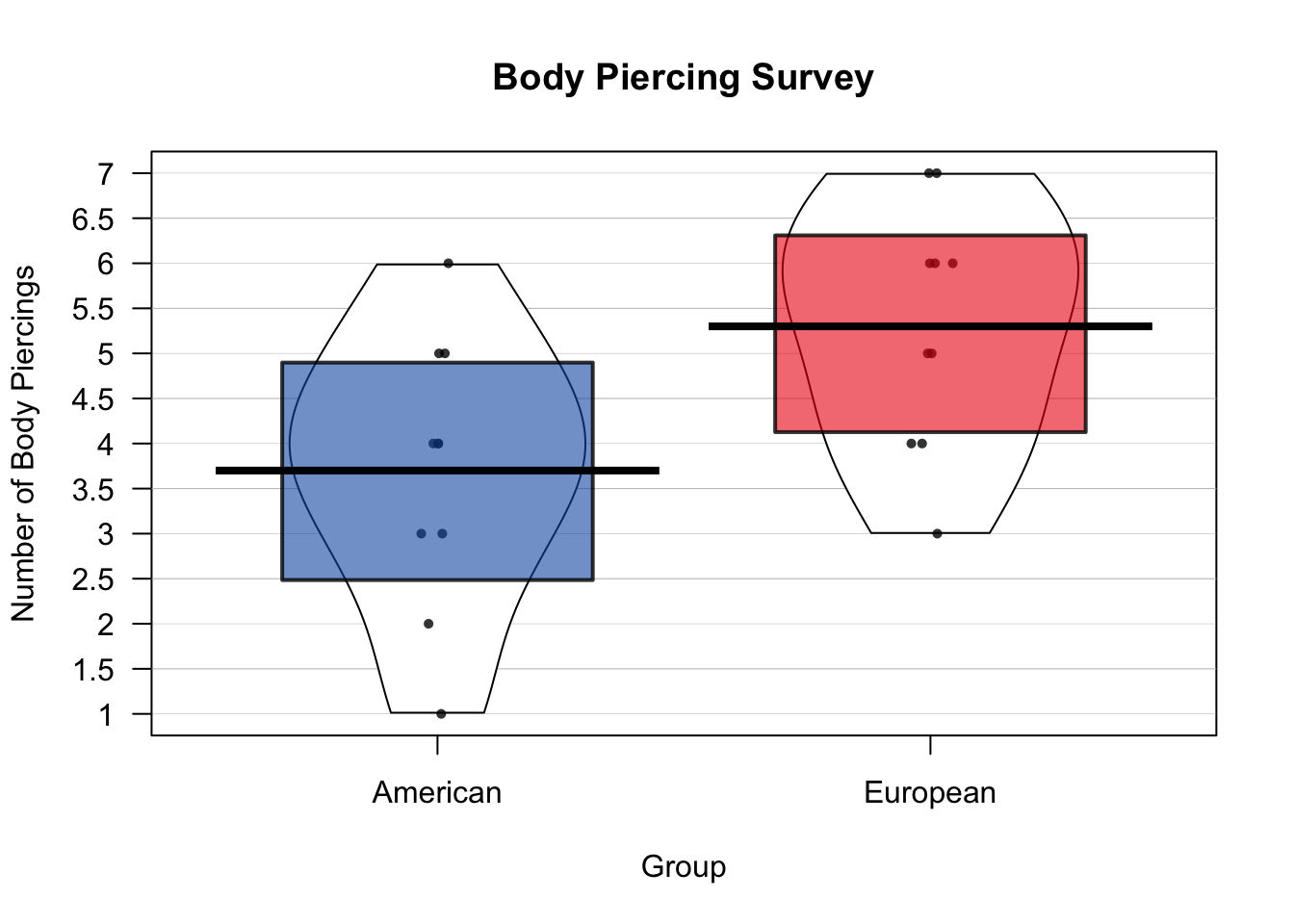
Figure 13.2: A Pirateplot of the body piercing data.
13.1.1 Null v Alternative Hypothesis
In null hypothesis tests, you always start with a null hypothesis. The specific null hypothesis you choose will depend on the type of question you are asking, but in general, the null hypothesis states that nothing is going on and everything is the same. For example, in our body piercing study, our null hypothesis is that American and European pirates have the same number of body piercings on average.
The alternative hypothesis is the opposite of the null hypothesis. In this case, our alternative hypothesis is that American and European pirates do not have the same number of piercings on average. We can have different types of alternative hypotheses depending on how specific we want to be about our prediction. We can make a 1-sided (also called 1-tailed) hypothesis, by predicting the direction of the difference between American and European pirates. For example, our alternative hypothesis could be that European pirates have more piercings on average than American pirates.
Alternatively, we could make a 2-sided (also called 2-tailed) alternative hypothesis that American and European pirates simply differ in their average number of piercings, without stating which group has more piercings than the other.
Once we’ve stated our null and alternative hypotheses, we collect data and then calculate descriptive statistics.
13.1.2 Descriptive statistics
Descriptive statistics (also called sample statistics) describe samples of data. For example, a mean, median, or standard deviation of a dataset is a descriptive statistic of that dataset. Let’s calculate some descriptive statistics on our body piercing survey American and European pirates using the summary() function:
# Pring descriptive statistics of the piercing data
summary(american.bp)
##    Min. 1st Qu.  Median    Mean 3rd Qu.    Max.
##     1.0     3.0     4.0     3.7     4.8     6.0
summary(european.bp)
##    Min. 1st Qu.  Median    Mean 3rd Qu.    Max.
##     3.0     4.2     5.5     5.3     6.0     7.0
Well, it looks like our sample of 10 American pirates had 3.7 body piercings on average, while our sample of 10 European pirates had 5.3 piercings on average. But is this difference large or small? Are we justified in concluding that American and European pirates in general differ in how many body piercings they have? To answer this, we need to calculate a test statistic
13.1.3 Test Statistics
An test statistic compares descriptive statistics, and determines how different they are. The formula you use to calculate a test statistics depends the type of test you are conducting, which depends on many factors, from the scale of the data (i.e.; is it nominal or interval?), to how it was collected (i.e.; was the data collected from the same person over time or were they all different people?), to how its distributed (i.e.; is it bell-shaped or highly skewed?).
For now, I can tell you that the type of data we are analyzing calls for a two-sample T-test. This test will take the descriptive statistics from our study, and return a test-statistic we can then use to make a decision about whether American and European pirates really differ. To calculate a test statistic from a two-sample t-test, we can use the t.test() function in R. Don’t worry if it’s confusing for now, we’ll go through it in detail shortly.
# Conduct a two-sided t-test comparing the vectors american.bp and european.bp
#  and save the results in an object called bp.test
bp.test <- t.test(x = american.bp,
                  y = european.bp,
                  alternative = "two.sided")

# Print the main results
bp.test
##
##  Welch Two Sample t-test
##
## data:  american.bp and european.bp
## t = -3, df = 20, p-value = 0.02
## alternative hypothesis: true difference in means is not equal to 0
## 95 percent confidence interval:
##  -2.93 -0.27
## sample estimates:
## mean of x mean of y
##       3.7       5.3
It looks like our test-statistic is -2.52. If there was really no difference between the groups of pirates, we would expect a test statistic close to 0. Because test-statistic is -2.52, this makes us think that there really is a difference. However, in order to make our decision, we need to get the p-value from the test.
13.1.4 p-value
The p-value is a probability that reflects how consistent the test statistic is with the hypothesis that the groups are actually the same. Or more formally, a p-value can be interpreted as follows:
13.1.4.1 Definition of a p-value: Assuming that there the null hypothesis is true (i.e.; that there is no difference between the groups), what is the probability that we would have gotten a test statistic as far away from 0 as the one we actually got?
For this problem, we can access the p-value as follows:
# What is the p-value from our t-test?
bp.test$p.value
## [1] 0.021
The p-value we got was 0.02, this means that, assuming the two populations of American and European pirates have the same number of body piercings on average, the probability that we would obtain a test statistic as large as -2.52 is 2.1% . This is very small, but is it small enough to decide that the null hypothesis is not true? It’s hard to say and there is no definitive answer. However, most pirates use a decision threshold of p < 0.05 to determine if we should reject the null hypothesis or not. In other words, if you obtain a p-value less than 0.05, then you reject the null hypothesis. Because our p-value of 0.02 is less than 0.05, we would reject the null hypothesis and conclude that the two populations are not be the same.
13.1.4.2 p-values are bullshit detectors against the null hypothesis

Figure 13.3: p-values are like bullshit detectors against the null hypothesis. The smaller the p-value, the more likely it is that the null-hypothesis (the idea that the groups are the same) is bullshit.
P-values sounds complicated – because they are (In fact, most psychology PhDs get the definition wrong). It’s very easy to get confused and not know what they are or how to use them. But let me help by putting it another way: a p-value is like a bullshit detector against the null hypothesis that goes off when the p-value is too small. If a p-value is too small, the bullshit detector goes off and says “Bullshit! There’s no way you would get data like that if the groups were the same!” If a p-value is not too small, the bullshit alarm stays silent, and we conclude that we cannot reject the null hypothesis.
13.1.4.3 How small of a p-value is too small?
Traditionally a p-value of 0.05 (or sometimes 0.01) is used to determine ‘statistical significance.’ In other words, if a p-value is less than .05, most researchers then conclude that the null hypothesis is false. However, .05 is not a magical number. Anyone who really believes that a p-value of .06 is much less significant than a p-value of 0.04 has been sniffing too much glue. However, in order to be consistent with tradition, I will adopt this threshold for the remainder of this chapter. That said, let me reiterate that a p-value threshold of 0.05 is just as arbitrary as a p-value of 0.09, 0.06, or 0.12156325234.
13.1.4.4 Does the p-value tell us the probability that the null hypothesis is true?
No!!! The p-value does not tell you the probability that the null hypothesis is true. In other words, if you calculate a p-value of .04, this does not mean that the probability that the null hypothesis is true is 4%. Rather, it means that if the null hypothesis was true, the probability of obtaining the result you got is 4%. Now, this does indeed set off our bullshit detector, but again, it does not mean that the probability that the null hypothesis is true is 4%.
Let me convince you of this with a short example. Imagine that you and your partner have been trying to have a baby for the past year. One day, your partner calls you and says “Guess what! I took a pregnancy test and it came back positive!! I’m pregnant!!” So, given the positive pregnancy test, what is the probability that your partner is really pregnant?

Figure 13.4: Despite what you may see in movies, men cannot get pregnant. And despite what you may want to believe, p-values do not tell you the probability that the null hypothesis is true!
Now, imagine that the pregnancy test your partner took gives incorrect results in 1% of cases. In other words, if you are pregnant, there is a 1% chance that the test will make a mistake and say that you are not pregnant. If you really are not pregnant, there is a 1% change that the test make a mistake and say you are pregnant.
Ok, so in this case, the null hypothesis here is that your partner is not pregnant, and the alternative hypothesis is that they are pregnant. Now, if the null hypothesis is true, then the probability that they would have gotten an (incorrect) positive test result is just 1%. Does this mean that the probability that your partner is not pregnant is only 1%.
No. Your partner is a man. The probability that the null hypothesis is true (i.e. that he is not pregnant), is 100%, not 1%. Your stupid boyfriend doesn’t understand basic biology and decided to buy an expensive pregnancy test anyway.
This is an extreme example of course – in most tests that you do, there will be some positive probability that the null hypothesis is false. However, in order to reasonably calculate an accurate probability that the null hypothesis is true after collecting data, you must take into account the prior probability that the null hypothesis was true before you collected data. The method we use to do this is with Bayesian statistics. We’ll go over Bayesian statistics in a later chapter.