11.9 Examples

Figure 11.17 shows a modified version of a scatterplot I call a balloonplot:

# Turn a boring scatterplot into a  balloonplot! 

# Create some random correlated data
x <- rnorm(50, mean = 50, sd = 10)
y <- x + rnorm(50, mean = 20, sd = 8)

# Set up the plotting space
plot(1, 
     bty = "n",
     xlim = c(0, 100),
     ylim = c(0, 100),
     type = "n", xlab = "", ylab = "", 
     main = "Turning a scatterplot into a balloon plot!")

# Add gridlines
grid()

# Add Strings with segments()
segments(x0 = x + rnorm(length(x), mean = 0, sd = .5), 
         y0 = y - 10, 
         x1 = x, 
         y1 = y, 
         col = gray(.1, .95),
         lwd = .5)

# Add balloons
points(x, y, 
       cex = 2, # Size of the balloons
       pch = 21, 
       col = "white", # white border
       bg = yarrr::piratepal("basel"))  # Filling color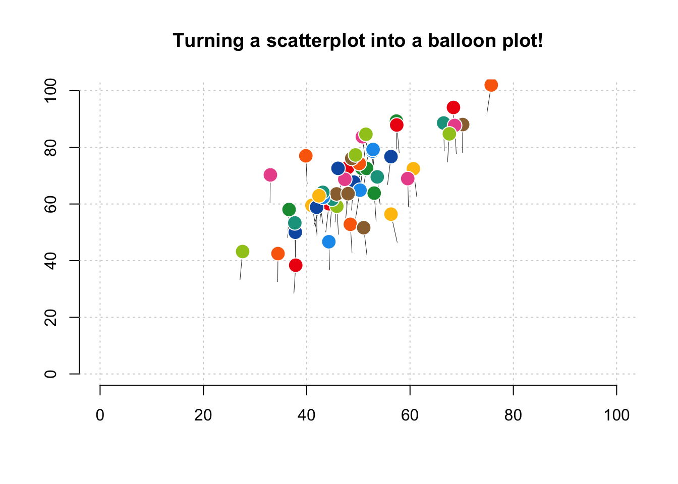

Figure 11.17: A balloon plot

You can use colors and point sizes in a scatterplot to represent third variables. In Figure 11.18, I’ll plot the relationship between pirate height and weight, but now I’ll make the size and color of each point reflect how many tattoos the pirate has

# Just the first 100 pirates
pirates.r <- pirates[1:100,]

plot(x = pirates.r$height,
     y = pirates.r$weight,
     xlab = "height",
     ylab = "weight",
     main = "Specifying point sizes and colors with a 3rd variable",
     cex = pirates.r$tattoos  / 8,          # Point size reflects how many tattoos they have
     col = gray(1 - pirates.r$tattoos / 20)) # color reflects tattoos

grid()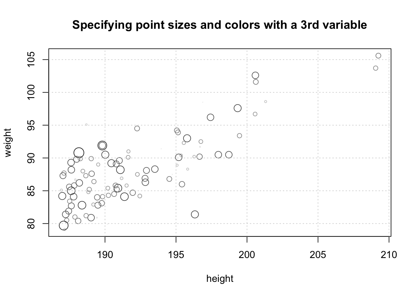

Figure 11.18: Specifying the size and color of points with a third variable.