12.3 Arranging plots with par(mfrow) and layout()

R makes it easy to arrange multiple plots in the same plotting space. The most common ways to do this is with the par(mfrow) parameter, and the layout() function. Let’s go over each in turn:

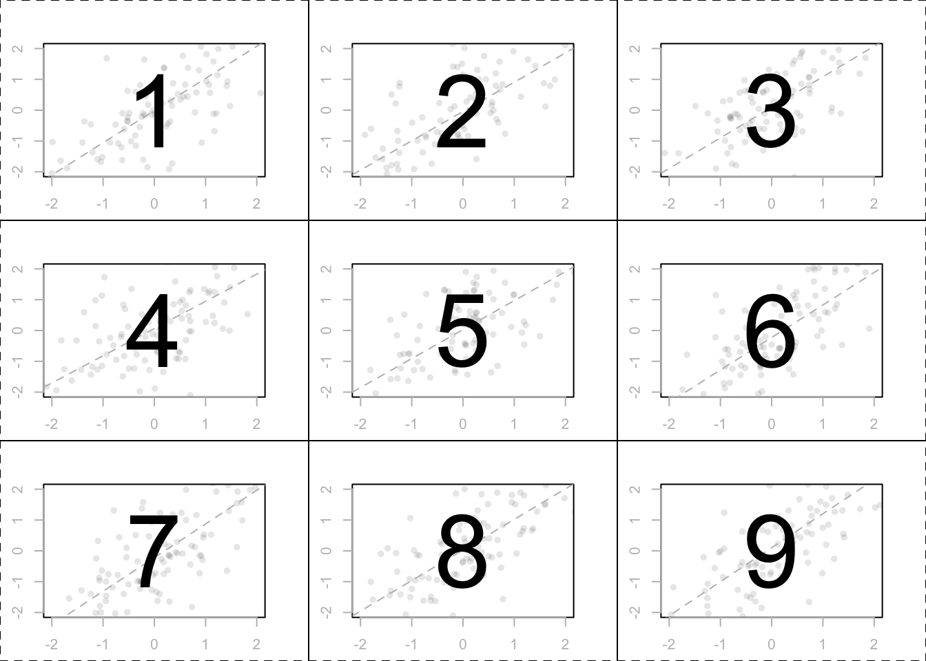
Figure 11.21: A 3 x 3 matrix of plotting regions created by par(mfrow = c(3, 3))

The mfrow and mfcol parameters allow you to create a matrix of plots in one plotting space. Both parameters take a vector of length two as an argument, corresponding to the number of rows and columns in the resulting plotting matrix. For example, the following code sets up a 3 x 3 plotting matrix.

par(mfrow = c(2, 2)) # Create a 2 x 2 plotting matrix
# The next 4 plots created will be plotted next to each other

# Plot 1
hist(rnorm(100))

# Plot 2
plot(pirates$weight, 
     pirates$height, pch = 16, col = gray(.3, .1))

# Plot 3
pirateplot(weight ~ Diet, 
           data = ChickWeight, 
           pal = "info", theme = 3)

# Plot 4
boxplot(weight ~ Diet, 
           data = ChickWeight)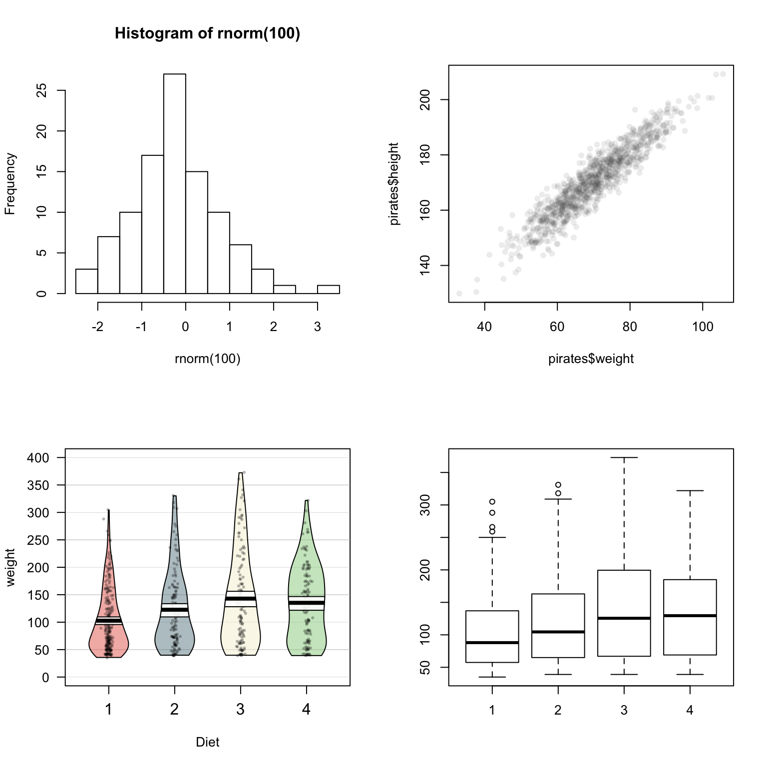

Figure 11.22: Arranging plots into a 2x2 matrix with par(mfrow = c(2, 2))

When you execute this code, you won’t see anything happen. However, when you execute your first high-level plotting command, you’ll see that the plot will show up in the space reserved for the first plot (the top left). When you execute a second high-level plotting command, R will place that plot in the second place in the plotting matrix - either the top middle (if using par(mfrow) or the left middle (if using par(mfcol)). As you continue to add high-level plots, R will continue to fill the plotting matrix.

So what’s the difference between par(mfrow) and par(mfcol)? The only difference is that while par(mfrow) puts sequential plots into the plotting matrix by row, par(mfcol) will fill them by column.

When you are finished using a plotting matrix, be sure to reset the plotting parameter back to its default state by running par(mfrow = c(1, 1)):

# Put plotting arrangement back to its original state
par(mfrow = c(1, 1))

12.3.1 Complex plot layouts with layout()

Argument	Description
mat	A matrix indicating the location of the next N figures in the global plotting space. Each value in the matrix must be 0 or a positive integer. R will plot the first plot in the entries of the matrix with 1, the second plot in the entries with 2,…
widths	A vector of values for the widths of the columns of the plotting space.
heights	A vector of values for the heights of the rows of the plotting space.

While par(mfrow) allows you to create matrices of plots, it does not allow you to create plots of different sizes. In order to arrange plots in different sized plotting spaces, you need to use the layout() function. Unlike par(mfrow), layout is not a plotting parameter, rather it is a function all on its own. The function can be a bit confusing at first, so I think it’s best to start with an example. Let’s say you want to place histograms next to a scatterplot: Let’s do this using layout:

We’ll begin by creating the layout matrix, this matrix will tell R in which order to create the plots:

layout.matrix <- matrix(c(0, 2, 3, 1), nrow = 2, ncol = 2)
layout.matrix
##      [,1] [,2]
## [1,]    0    3
## [2,]    2    1

Looking at the values of layout.matrix, you can see that we’ve told R to put the first plot in the bottom right, the second plot on the bottom left, and the third plot in the top right. Because we put a 0 in the first element, R knows that we don’t plan to put anything in the top left area.

Now, because our layout matrix has two rows and two columns, we need to set the widths and heights of the two columns. We do this using a numeric vector of length 2. I’ll set the heights of the two rows to 1 and 2 respectively, and the widths of the columns to 1 and 2 respectively. Now, when I run the code layout.show(3), R will show us the plotting region we set up:

layout.matrix <- matrix(c(2, 1, 0, 3), nrow = 2, ncol = 2)

layout(mat = layout.matrix,
       heights = c(1, 2), # Heights of the two rows
       widths = c(2, 2)) # Widths of the two columns

layout.show(3)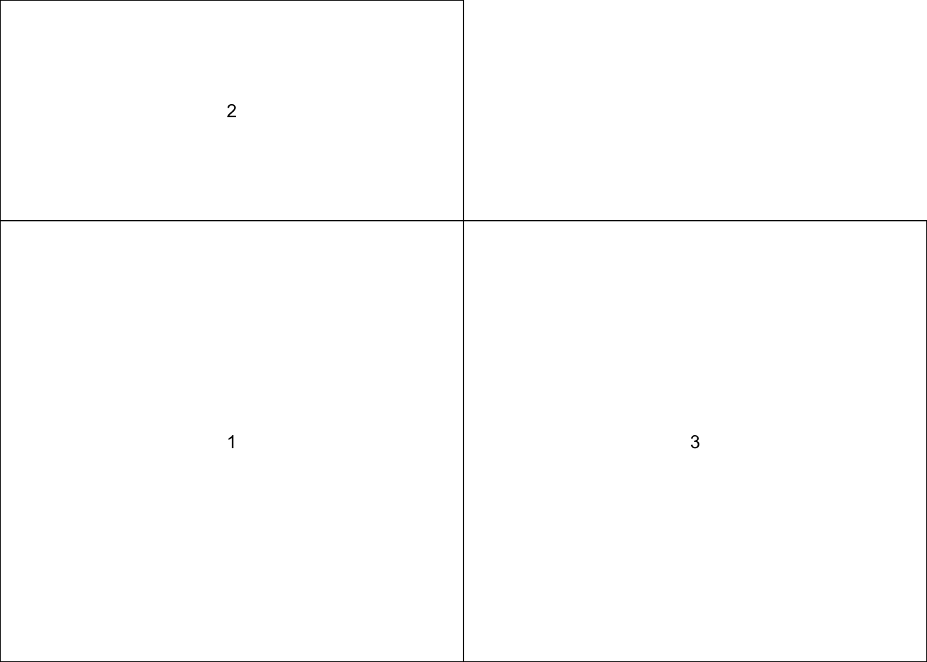

Figure 11.23: A plotting layout created by setting a layout matrix with two rows and two columns. The first row has a height of 1, and the second row has a hight of 2. Both columns have the same width of 2.

Now we’re ready to put the plots together

# Set plot layout
layout(mat = matrix(c(2, 1, 0, 3), 
                        nrow = 2, 
                        ncol = 2),
       heights = c(1, 2),    # Heights of the two rows
       widths = c(2, 1))     # Widths of the two columns

# Plot 1: Scatterplot
par(mar = c(5, 4, 0, 0))
plot(x = pirates$height, 
     y = pirates$weight,
     xlab = "height", 
     ylab = "weight", 
     pch = 16, 
     col = yarrr::piratepal("pony", trans = .7))

# Plot 2: Top (height) boxplot
par(mar = c(0, 4, 0, 0))
boxplot(pirates$height, xaxt = "n",
        yaxt = "n", bty = "n", yaxt = "n",
        col = "white", frame = FALSE, horizontal = TRUE)

# Plot 3: Right (weight) boxplot
par(mar = c(5, 0, 0, 0))
boxplot(pirates$weight, xaxt = "n",
        yaxt = "n", bty = "n", yaxt = "n",
        col = "white", frame = F)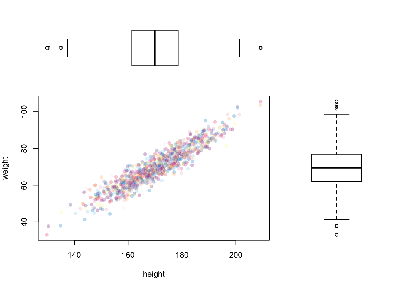

Figure 11.24: Adding boxplots to margins of a scatterplot with layout().