15.2 Linear regression with lm()
| Argument | Description |
|---|---|
formula |
A formula in the form y ~ x1 + x2 + ... where y is the dependent variable, and x1, x2, … are the independent variables. If you want to include all columns (excluding y) as independent variables, just enter y ~ . |
data |
The dataframe containing the columns specified in the formula. |
To estimate the beta weights of a linear model in R, we use the lm() function. The function has three key arguments: formula, and data
15.2.1 Estimating the value of diamonds with lm()
We’ll start with a simple example using a dataset in the yarrr package called . The dataset includes data on 150 diamonds sold at an auction. Here are the first few rows of the dataset:
library(yarrr)
head(diamonds)
##   weight clarity color value value.lm weight.c clarity.c value.g190
## 1    9.3    0.88     4   182      186    -0.55     -0.12      FALSE
## 2   11.1    1.05     5   191      193     1.20      0.05       TRUE
## 3    8.7    0.85     6   176      183    -1.25     -0.15      FALSE
## 4   10.4    1.15     5   195      194     0.53      0.15       TRUE
## 5   10.6    0.92     5   182      189     0.72     -0.08      FALSE
## 6   12.3    0.44     4   183      183     2.45     -0.56      FALSE
##   pred.g190
## 1     0.163
## 2     0.821
## 3     0.030
## 4     0.846
## 5     0.445
## 6     0.087
Our goal is to come up with a linear model we can use to estimate the value of each diamond (DV = value) as a linear combination of three independent variables: its weight, clarity, and color. The linear model will estimate each diamond’s value using the following equation:
\(\beta_{Int} + \beta_{weight} \times weight + \beta_{clarity} \times clarity + \beta_{color} \times color\)
where \(\beta_{weight}\) is the increase in value for each increase of 1 in weight, \(\beta_{clarity}\) is the increase in value for each increase of 1 in clarity (etc.). Finally, \(\beta_{Int}\) is the baseline value of a diamond with a value of 0 in all independent variables.
To estimate each of the 4 weights, we’ll use lm(). Because value is the dependent variable, we’ll specify the formula as formula = value ~ weight + clarity + color. We’ll assign the result of the function to a new object called diamonds.lm:
# Create a linear model of diamond values
#   DV = value, IVs = weight, clarity, color

diamonds.lm <- lm(formula = value ~ weight + clarity + color,
                  data = diamonds)
To see the results of the regression analysis, including estimates for each of the beta values, we’ll use the summary() function:
# Print summary statistics from diamond model
summary(diamonds.lm)
##
## Call:
## lm(formula = value ~ weight + clarity + color, data = diamonds)
##
## Residuals:
##     Min      1Q  Median      3Q     Max
## -10.405  -3.547  -0.113   3.255  11.046
##
## Coefficients:
##             Estimate Std. Error t value Pr(>|t|)
## (Intercept)  148.335      3.625   40.92   <2e-16 ***
## weight         2.189      0.200   10.95   <2e-16 ***
## clarity       21.692      2.143   10.12   <2e-16 ***
## color         -0.455      0.365   -1.25     0.21
## ---
## Signif. codes:  0 '***' 0.001 '**' 0.01 '*' 0.05 '.' 0.1 ' ' 1
##
## Residual standard error: 4.7 on 146 degrees of freedom
## Multiple R-squared:  0.637,  Adjusted R-squared:  0.63
## F-statistic: 85.5 on 3 and 146 DF,  p-value: <2e-16
Here, we can see from the summary table that the model estimated \(\beta_{Int}\) (the intercept), to be 148.34, \(\beta_{weight}\) to be 2.19, \(\beta_{clarity}\) to be 21.69, and , \(\beta_{color}\) to be -0.45. You can see the full linear model in Figure 15.2:
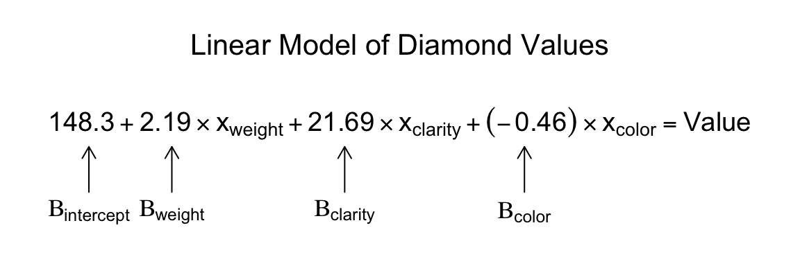
Figure 15.2: A linear model estimating the values of diamonds based on their weight, clarity, and color.
You can access lots of different aspects of the regression object. To see what’s inside, use names()
# Which components are in the regression object?
names(diamonds.lm)
##  [1] "coefficients"  "residuals"     "effects"       "rank"
##  [5] "fitted.values" "assign"        "qr"            "df.residual"
##  [9] "xlevels"       "call"          "terms"         "model"
For example, to get the estimated coefficients from the model, just access the coefficients attribute:
# The coefficients in the diamond model
diamonds.lm$coefficients
## (Intercept)      weight     clarity       color
##    148.3354      2.1894     21.6922     -0.4549
If you want to access the entire statistical summary table of the coefficients, you just need to access them from the summary object:
# Coefficient statistics in the diamond model
summary(diamonds.lm)$coefficients
##             Estimate Std. Error t value  Pr(>|t|)
## (Intercept) 148.3354     3.6253  40.917 7.009e-82
## weight        2.1894     0.2000  10.948 9.706e-21
## clarity      21.6922     2.1429  10.123 1.411e-18
## color        -0.4549     0.3646  -1.248 2.141e-01
15.2.2 Getting model fits with fitted.values
To see the fitted values from a regression object (the values of the dependent variable predicted by the model), access the fitted.values attribute from a regression object with $fitted.values.
Here, I’ll add the fitted values from the diamond regression model as a new column in the diamonds dataframe:
# Add the fitted values as a new column in the dataframe
diamonds$value.lm <- diamonds.lm$fitted.values

# Show the result
head(diamonds)
##   weight clarity color value value.lm weight.c clarity.c value.g190
## 1   9.35    0.88     4 182.5    186.1  -0.5511   -0.1196      FALSE
## 2  11.10    1.05     5 191.2    193.1   1.1989    0.0504       TRUE
## 3   8.65    0.85     6 175.7    183.0  -1.2511   -0.1496      FALSE
## 4  10.43    1.15     5 195.2    193.8   0.5289    0.1504       TRUE
## 5  10.62    0.92     5 181.6    189.3   0.7189   -0.0796      FALSE
## 6  12.35    0.44     4 182.9    183.1   2.4489   -0.5596      FALSE
##   pred.g190
## 1   0.16252
## 2   0.82130
## 3   0.03008
## 4   0.84559
## 5   0.44455
## 6   0.08688
According to the model, the first diamond, with a weight of 9.35, a clarity of 0.88, and a color of 4 should have a value of 186.08. As we can see, this is not far off from the true value of 182.5.
You can use the fitted values from a regression object to plot the relationship between the true values and the model fits. If the model does a good job in fitting the data, the data should fall on a diagonal line:
# Plot the relationship between true diamond values
#   and linear model fitted values

plot(x = diamonds$value,                          # True values on x-axis
     y = diamonds.lm$fitted.values,               # fitted values on y-axis
     xlab = "True Values",
     ylab = "Model Fitted Values",
     main = "Regression fits of diamond values")

abline(b = 1, a = 0)                             # Values should fall around this line!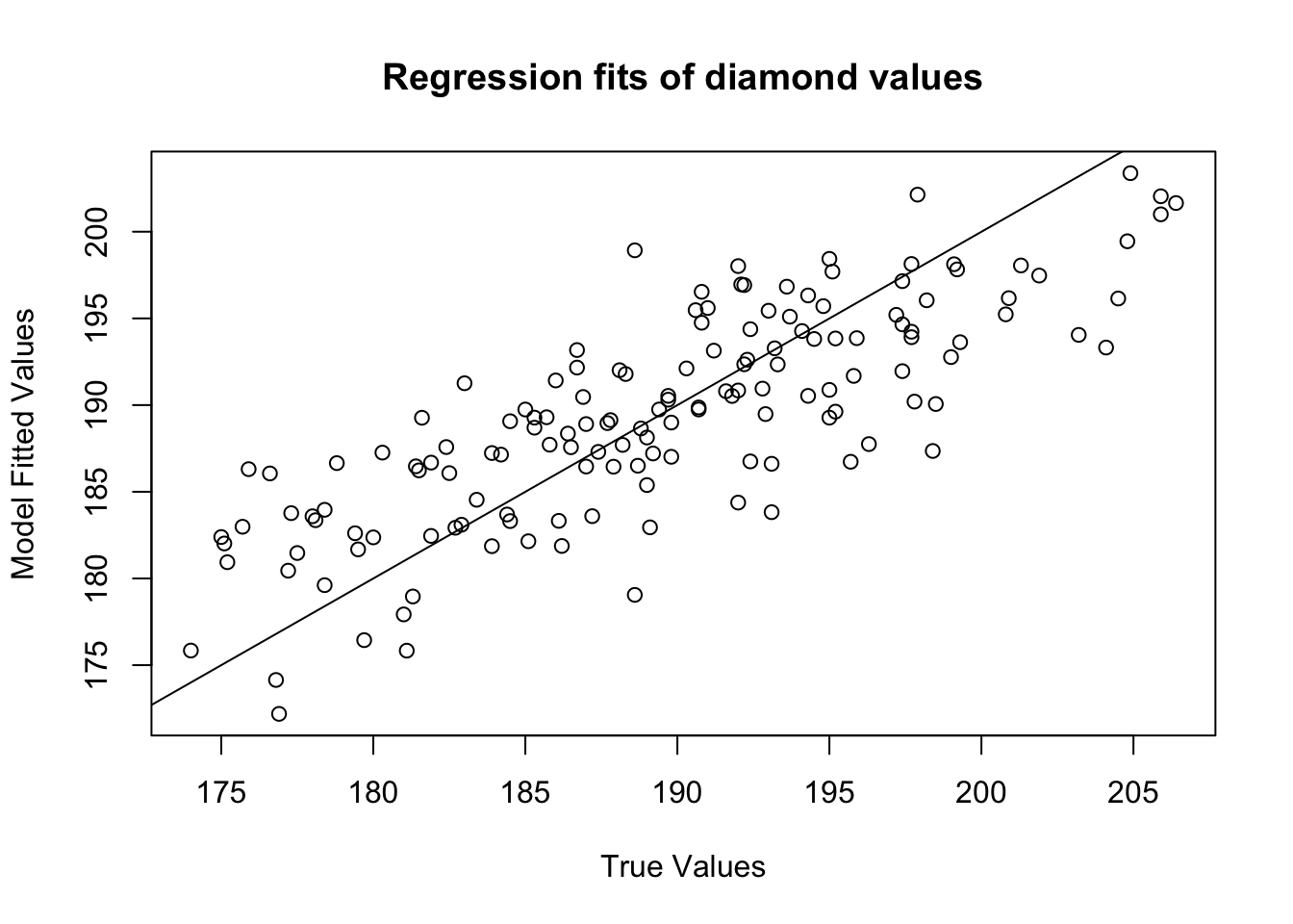
15.2.3 Using predict() to predict new data from a model
Once you have created a regression model with lm(), you can use it to easily predict results from new datasets using the predict() function.
For example, let’s say I discovered 3 new diamonds with the following characteristics:
| weight | clarity | color |
|---|---|---|
| 20 | 1.5 | 5 |
| 10 | 0.2 | 2 |
| 15 | 5.0 | 3 |
I’ll use the predict() function to predict the value of each of these diamonds using the regression model diamond.lm that I created before. The two main arguments to predict() are object – the regression object we’ve already defined), and newdata – the dataframe of new data. Warning! The dataframe that you use in the newdata argument to predict() must have column names equal to the names of the coefficients in the model. If the names are different, the predict() function won’t know which column of data applies to which coefficient and will return an error.
# Create a dataframe of new diamond data
diamonds.new <- data.frame(weight = c(12, 6, 5),
                           clarity = c(1.3, 1, 1.5),
                           color = c(5, 2, 3))

# Predict the value of the new diamonds using
#  the diamonds.lm regression model
predict(object = diamonds.lm,     # The regression model
        newdata = diamonds.new)   # dataframe of new data
##     1     2     3
## 200.5 182.3 190.5
This result tells us the the new diamonds are expected to have values of 200.5, 182.3, and 190.5 respectively according to our regression model.
15.2.4 Including interactions in models: y ~ x1 * x2
To include interaction terms in a regression model, just put an asterix (*) between the independent variables. For example, to create a regression model on the diamonds data with an interaction term between weight and clarity, we’d use the formula formula = value ~ weight * clarity:
# Create a regression model with interactions between
#   IVS weight and clarity
diamonds.int.lm <- lm(formula = value ~ weight * clarity,
                      data = diamonds)

# Show summary statistics of model coefficients
summary(diamonds.int.lm)$coefficients
##                Estimate Std. Error t value  Pr(>|t|)
## (Intercept)    157.4721     10.569 14.8987 4.170e-31
## weight           0.9787      1.070  0.9149 3.617e-01
## clarity          9.9245     10.485  0.9465 3.454e-01
## weight:clarity   1.2447      1.055  1.1797 2.401e-01
15.2.5 Center variables before computing interactions!
Hey what happened? Why are all the variables now non-significant? Does this mean that there is really no relationship between weight and clarity on value after all? No. Recall from your second-year pirate statistics class that when you include interaction terms in a model, you should always center the independent variables first. Centering a variable means simply subtracting the mean of the variable from all observations.
In the following code, I’ll repeat the previous regression, but first I’ll create new centered variables weight.c and clarity.c, and then run the regression on the interaction between these centered variables:
# Create centered versions of weight and clarity
diamonds$weight.c <- diamonds$weight - mean(diamonds$weight)
diamonds$clarity.c <- diamonds$clarity - mean(diamonds$clarity)

# Create a regression model with interactions of centered variables
diamonds.int.lm <- lm(formula = value ~ weight.c * clarity.c,
                      data = diamonds)

# Print summary
summary(diamonds.int.lm)$coefficients
##                    Estimate Std. Error t value   Pr(>|t|)
## (Intercept)         189.402     0.3831  494.39 2.908e-237
## weight.c              2.223     0.1988   11.18  2.322e-21
## clarity.c            22.248     2.1338   10.43  2.272e-19
## weight.c:clarity.c    1.245     1.0551    1.18  2.401e-01
Hey that looks much better! Now we see that the main effects are significant and the interaction is non-significant.
15.2.6 Getting an ANOVA from a regression model with aov()
Once you’ve created a regression object with lm() or glm(), you can summarize the results in an ANOVA table with aov():
# Create ANOVA object from regression
diamonds.aov <- aov(diamonds.lm)

# Print summary results
summary(diamonds.aov)
##              Df Sum Sq Mean Sq F value Pr(>F)
## weight        1   3218    3218  147.40 <2e-16 ***
## clarity       1   2347    2347  107.53 <2e-16 ***
## color         1     34      34    1.56   0.21
## Residuals   146   3187      22
## ---
## Signif. codes:  0 '***' 0.001 '**' 0.01 '*' 0.05 '.' 0.1 ' ' 1